
Chapter 7
Time–Space Scheduling in the MapReduce Framework
Zhuo Tang, Ling Qi, Lingang Jiang, Kenli Li, and Keqin Li
Abstract
As data are the basis of information systems, using Hadoop to rapidly extract useful information from massive data of an enterprise has become an efficient method for programmers in the process of application development. This chapter introduces the MapReduce framework, an excellent distributed and parallel computing model. For the increasing data and cluster scales, to avoid scheduling delays, scheduling skews, poor system utilization, and low degrees of parallelism, some improved methods that focus on the time and space scheduling of reduce tasks in MapReduce are proposed in this chapter. Through analyzing the MapReduce scheduling mechanism, this chapter first illustrates the reasons for system slot resource wasting, which results in reduce tasks waiting around, and proposes the development of a method detailing the start times of reduce tasks dynamically according to each job context. And then, in order to mitigate network traffic and improve the performance of Hadoop, this chapter addresses several optimizing algorithms to solve the problems of reduce placement. It makes a Hadoop reduce task scheduler aware of partitions’ network locations and sizes. Finally, as the implementation, a parallel biomedical data processing model using the MapReduce framework is presented as an application of the proposed methods.
7.1 INTRODUCTION
Data are representations of information, the information content of data is generally believed to be valuable, and data form the basis of information systems. Using computers to process data, extracting information is a basic function of information systems. In today’s highly information-oriented society, the web can be said to be currently the largest information system, of which the data are massive, diverse, heterogeneous, and dynamically changing. Using Hadoop to rapidly extract useful information from the massive data of an enterprise has become an efficient method for programmers in the process of application development.
The significance of Big Data is to analyze people’s behavior, intentions, and preferences in the growing and popular social networks. It is also to process data with nontraditional structures and to explore their meanings. Big Data is often used to describe a company’s large amount of unstructured and semistructured data. Using analysis to create these data in a relational database for downloading will require too much time and money. Big Data analysis and cloud computing are often linked together, because real-time analysis of large data requires a framework similar to MapReduce to assign work to hundreds or even thousands of computers. After several years of criticism, questioning, discussion, and speculation, Big Data finally ushered in the era belonging to it.
Hadoop presents MapReduce as an analytics engine, and under the hood, it uses a distributed storage layer referred to as the Hadoop distributed file system (HDFS). As an open-source implementation of MapReduce, Hadoop is, so far, one of the most successful realizations of large-scale data-intensive cloud computing platforms. It has been realized that when and where to start the reduce tasks are the key problems to enhance MapReduce performance.
For time scheduling in MapReduce, the existing work may result in a block of reduce tasks. Especially when the map tasks’ output is large, the performance of a MapReduce task scheduling algorithm will be influenced seriously. Through analysis for the current MapReduce scheduling mechanism, Section 7.3 illustrates the reasons for system slot resource wasting, which results in reduce tasks waiting around. Then, the section proposes a self-adaptive reduce task scheduling policy for reduce tasks’ start times in the Hadoop platform. It can decide the start time point of each reduce task dynamically according to each job context, including the task completion time and the size of the map output.
Meanwhile, another main performance bottleneck is caused by all-to-all communications between mappers and reducers, which may saturate the top-of-rack switch and inflate job execution time. The bandwidth between two nodes is dependent on their relative locations in the network topology. Thus, moving data repeatedly to remote nodes becomes the bottleneck. For this bottleneck, reducing cross-rack communication will improve job performance. Current research proves that moving a task is more efficient than moving data [1], especially in the Hadoop distributed environment, where data skews are widespread.
Data skew is an actual problem to be resolved for MapReduce. The existing Hadoop reduce task scheduler is not only locality unaware but also partitioning skew unaware. The parallel and distributed computation features may cause some unforeseen problems. Data skew is a typical such problem, and the high runtime complexity amplifies the skew and leads to highly varying execution times of the reducers. Partitioning skew causes shuffle skew, where some reduce tasks receive more data than others. The shuffle skew problem can degrade performance, because a job might get delayed by a reduce task fetching large input data. In the presence of data skew, we can use a reducer placement method to minimize all-to-all communications between mappers and reducers, whose basic idea is to place related map and reduce tasks on the same node, cluster, or rack.
Section 7.4 addresses space scheduling in MapReduce. We analyze the source of data skew and conclude that partitioning skew exists within certain Hadoop applications. The node at which a reduce task is scheduled can effectively mitigate the shuffle skew problem. In these cases, reducer placement can decrease the traffic between mappers and reducers and upgrade system performance. Some algorithms are released, which synthesize the network locations and sizes of reducers’ partitions in their scheduling decisions in order to mitigate network traffic and improve MapReduce performance. Overall, Section 7.4 introduces several ways to avoid scheduling delay, scheduling skew, poor system utilization, and low degree of parallelism.
Some typical applications are discussed in this chapter. At present, there is an enormous quantity of biomedical literature, and it continues to increase at high speed. People urgently need some automatic tools to process and analyze the biomedical literature. In the current methods, the model training time increases sharply when dealing with large-scale training samples. How to increase the efficiency of named entity recognition (NER) in biomedical Big Data becomes one of the key problems in biomedical text mining. For the purposes of improving the recognition performance and reducing the training time, through implementing the model training process based on MapReduce, Section 7.5 proposes an optimization method for two-phase recognition using conditional random fields (CRFs) with some new feature sets.
7.2 OVERVIEW OF Big Data PROCESSING ARCHITECTURE
MapReduce is an excellent model for distributed computing, introduced by Google in 2004 [2]. It has emerged as an important and widely used programming model for distributed and parallel computing, due to its ease of use, generality, and scalability. Among its open-source implementation versions, Hadoop has been widely used in industry around the whole world [3]. It has been applied to production environments, such as Google, Yahoo, Amazon, Facebook, and so on. Because of the short development time, Hadoop can be improved in many aspects, such as the problems of intermediate data management and reduce task scheduling [4].
As shown in Figure 7.1, map and reduce are two sections in a MapReduce scheduling algorithm. In Hadoop, each task contains three function phases, that is, copy, sort, and reduce [5]. The goal of the copy phase is to read the map tasks’ output. The sort phase is to sort the intermediate data, which are the output from map tasks and will be the input to the reduce phase. Finally, the eventual results are produced through the reduce phase, where the copy and sort phases are to preprocess the input data of the reduce phase. In real applications, copying and sorting may cost a considerable amount of time, especially in the copy phase. In the theoretical model, the reduce functions start only if all map tasks are finished [6]. However, in the Hadoop implementation, all copy actions of reduce tasks will start when the first map action is finished [7]. But in slot duration, if there is any map task still running, the copy actions will wait around. This will lead to the waste of reduce slot resources.
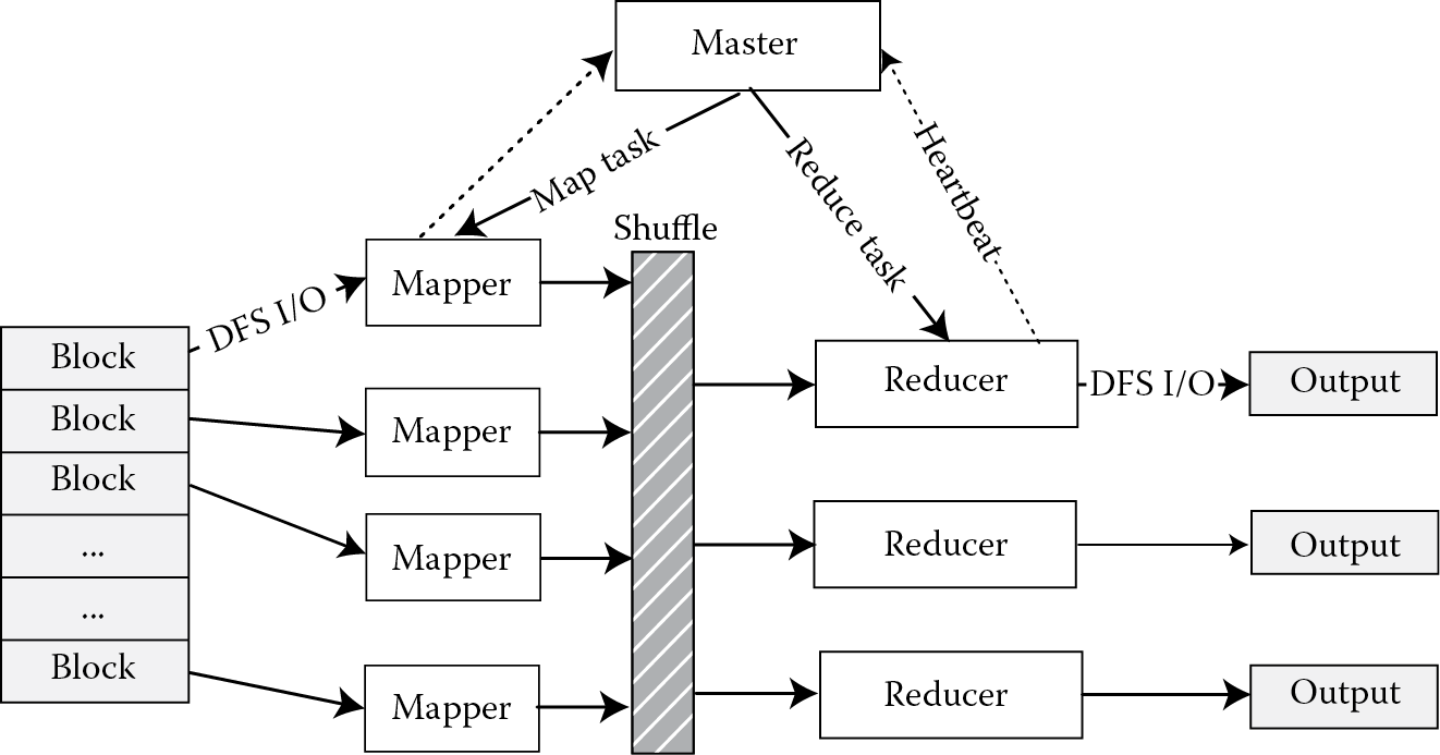
In traditional MapReduce scheduling, reduce tasks should start when all the map tasks are completed. In this way, the output of map tasks should be read and written to the reduce tasks in the copy process [8]. However, through the analysis of the slot resource usage in the reduce process, this chapter focuses on the slot idling and delay. In particular, when the map tasks’ output becomes large, the performance of MapReduce scheduling algorithms will be influenced seriously [9]. When multiple tasks are running, inappropriate scheduling of the reduce tasks will lead to the situation where other jobs in the system cannot be scheduled in a timely manner. These are the stumbling blocks of Hadoop popularization.
A user needs to serve two functions in the Hadoop framework, that is, mapper and reducer, to process data. Mappers produce a set of files and send it to all the reducers. Reducers will receive files from all the mappers, which is an all-to-all communication model. Hadoop runs in a data center environment in which machines are organized in racks. Cross-rack communication happens if a mapper and a reducer reside in different racks. Every cross-rack communication needs to travel through the root switch, and hence, the all-to-all communication model becomes a bottleneck.
This chapter points out the main affecting factors for the system performance in the MapReduce framework. The solutions to these problems constitute the content of the proposed time–space scheduling algorithms. In Section 7.3, we present a self-adaptive reduce task scheduling algorithm to resolve the problem of slot idling and waste. In Section 7.4, we analyze the source of data skew in MapReduce and introduce some methods to minimize cross-rack communication and MapReduce traffic. To show the application of this advanced MapReduce framework, in Section 7.5, we describe a method to provide the parallelization of model training in NER in biomedical Big Data mining.
7.3 SELF-ADAPTIVE REDUCE TASK SCHEDULING
7.3.1 Problem Analysis
Through studying reduce task scheduling in the Hadoop platform, this chapter proposes an optimizing policy called self-adaptive reduce scheduling (SARS) [10]. This method can decrease the waiting around of copy actions and enhance the performance of the whole system. Through analyzing the details of the map and reduce two-phase scheduling process at the runtime of the MapReduce tasks [8], SARS can determine the start time point of each reduce task dynamically according to each job’s context, such as the task completion time, the size of the map output [11], and so forth. This section makes the following contributions: (1) analysis of the current MapReduce scheduling mechanism and illustration of the reasons for system slot resource wasting, which results in reduce tasks waiting around; (2) development of a method to determine the start times of reduce tasks dynamically according to each job context, including the task completion time and the size of the map output; and (3) description of an optimizing reduce scheduling algorithm, which decreases the reduce completion time and system average response time in a Hadoop platform.
Hadoop allows the user to configure the job, submit it, control its execution, and query the state. Every job consists of independent tasks, and each task needs to have a system slot to run. Figure 7.2 shows the time delay and slot resource waste problem in reduce task scheduling. Through Figure 7.2, we can know that Job1 and Job2 are the current running jobs, and at the initial time, each job is allocated two map slots to run respective tasks. Since the execution time of each task is not the same, as shown in Figure 7.2, Job2 finishes its map tasks at time t2. Because the reduce tasks will begin once any map task finishes, from the duration t1 to t2, there are two reduce tasks from Job1 and Job2, which are running respectively. As indicated in Figure 7.2, at time t3, when all the reduce tasks of Job2 are finished, two new reduce tasks from Job1 are started. Now all the reduce slot resources are taken up by Job1. As shown in Figure 7.2, at the moment t4, when Job3 starts, two idle map slots can be assigned to it, and the reduce tasks from this job will then start. However, we can find that all reduce slots are already occupied by Job1, and the reduce tasks from Job3 have to wait for slot release.
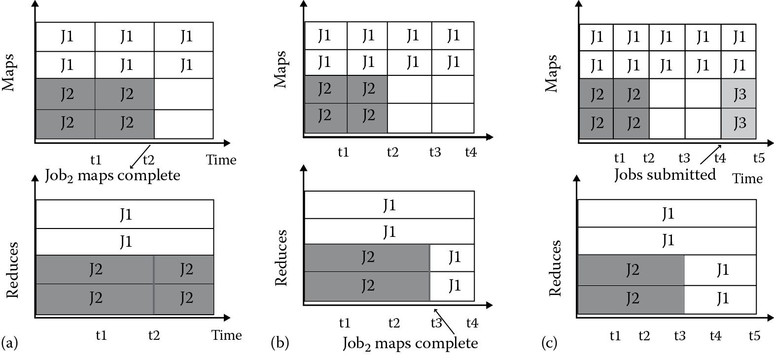
Performance of the policies with respect to various graph sizes. (a) Job2 map tasks finished. (b) Job2 reduce tasks finished. (c) Job3 submitted.
The root cause of this problem is that the reduce task of Job3 must wait for all the reduce tasks of Job1 to be completed, as Job1 takes up all the reduce slots and the Hadoop system does not support preemptive action acquiescently. In early algorithm design, a reduce task can be scheduled once any map tasks are finished [12]. One of the benefits is that the reduce tasks can copy the output of the map tasks as soon as possible. But reduce tasks will have to wait before all map tasks are finished, and the pending tasks will always occupy the slot resources, so that other jobs that finish the map tasks cannot start the reduce tasks. All in all, this will result in long waiting of reduce tasks and will greatly increase the delay of Hadoop jobs.
In practical applications, there are often different jobs running in a shared cluster environment, which are from multiple users at the same time. If the situation described in Figure 7.2 appears among the different users at the same time, and the reduce slot resources are occupied for a long time, the submitted jobs from other users will not be pushed ahead until the slots are released. Such inefficiency will extend the average response time of a Hadoop system, lower the resource utilization rate, and affect the throughput of a Hadoop cluster.
7.3.2 Runtime Analysis of MapReduce Jobs
Through the analysis in Section 7.3.1, one method to optimize the MapReduce tasks is to select an adaptive time to schedule the reduce tasks. By this means, we can avoid the reduce tasks’ waiting around and enhance the resource utilization rate. This section proposes a self-adaptive reduce task scheduling policy, which gives a method to estimate the start time of a task, instead of the traditional mechanism where reduce tasks are started once any map task is completed.
The reduce process can be divided into the following several phases. First, reduce tasks request to read the output data of map tasks in the copy phase, this will bring data transmissions from map tasks to reduce tasks. Next, in the sort process, these intermediate data are ordered by merging, and the data are distributed in different storage locations. One type is the data in memory. When the data are read from the various maps at the same time, the data set should be merged as the same keys. The other type is data as the circle buffer. Because the memory belonging to the reduce task is limited, the data in the buffer should be written to disks regularly in advance.
In this way, subsequent data which are written into the disk earlier need to be merged, so-called external sorting. The external sorting needs to be executed several times if the number of map tasks is large in the practical works. The copy and sort processes are customarily called the shuffle phase. Finally, after finishing the copy and sort processes, the subsequent functions start, and the reduce tasks can be scheduled to the compute nodes.
7.3.3 A Method of Reduce Task Start-Time Scheduling
Because Hadoop employs a greedy strategy to schedule the reduce tasks, to schedule the reduce tasks fastest, as described in Section 7.3.1, some reduce tasks will always take up the system resources without actually performing operations for a long time. Reduce task start time is determined by the advanced algorithm SARS. In this method, the start times of the reduce tasks are delayed for a certain duration to lessen the utilization of system resources. The SARS algorithm schedules the reduce tasks at a special moment, when some map tasks are finished but not all. By this means, how to select an optimal time point to start the reduce scheduling is the key problem of the algorithm. Distinctly, the optimum point can minimize the system delay and maximize the resource utilization.
As shown in Figure 7.3, assuming that Job1 has 16 map tasks and 1 reduce task, and there are 4 map slots and only 1 reduce slot in this cluster system. Figure 7.3 and Figure 7.4 describe the time constitution of the life cycle for a special job:
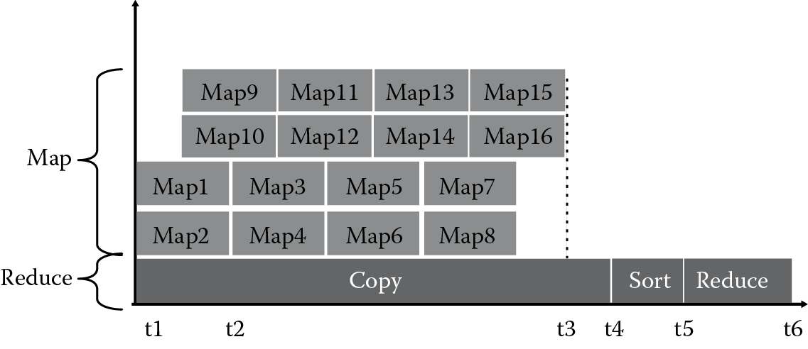
(FTlm − STfm) + (FTcp − FTlm) + (FTlr + STsr). (7.1)
The denotations in Equation 7.1 are defined as follows. FTlm is the completion time of the last map task; STfm is the start time of the first map task; FTcp is the finish time of the copy phase; FTlr is the finish time of reduce; and STsr is the start time of reduce sort.
In Figure 7.3, t1 is the start time of Map1, Map2, and the reduce task. During t1 to t3, the main work of the reduce task is to copy the output from Map1 to Map14. The output of Map15 and Map16 will be copied by the reduce task from t3 to t4. The duration from t4 to t5 is called the sort stage, which ranks the intermediate results according to the key values. The reduce function is called at time t5, which continues from t5 to t6. Because during t1 to t3, in the copy phase, the reduce task only copies the output data intermittently, once any map task is completed, for the most part, it is always waiting around. We hope to make the copy operations completed at a concentrated duration, which can decrease the waiting time of the reduce tasks.
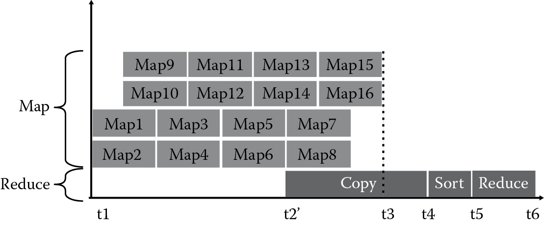
As Figure 7.4 shows, if we can start the reduce tasks at t2′, which can be calculated using the following equations, and make sure these tasks can be finished before t6, then during t1 to t2′, the slots can be used by any other reduce tasks. But if we let the copy operation start at t3, because the output of all map tasks should be copied from t3, delay will be produced in this case. As shown in Figure 7.3, the copy phase starts at t2, which just collects the output of the map tasks intermittently. By contrast, the reduce task’s waiting time is decreased obviously in Figure 7.4, in which case the copy operations are started at t2′.
The SARS algorithm works by delaying the reduce processes. The reduce tasks are scheduled when part but not all of the map tasks are finished. For a special key value, if we assume that there are s map slots and m map tasks in the current system, and the completion time and the size of output data of each map task are denoted as t_mapi and m_outj, respectively, where i, j ∈ [1,m]. Then, we can know that the data size of the map tasks can be calculated as
. (7.2)
In order to predict the time required to transmit the data, we define the speed of the data transmission from the map tasks to the reduce tasks as transSpeed in the cluster environment, and the number of concurrent copy threads with reduce tasks is denoted as copyThread. We denote the start time of the first map task and the first reduce task as startmap and startreduce, respectively. Therefore, the optimal start time of reduce tasks can be determined by the following equation:
(7.3)
As shown by time t2′ in Figure 7.4, the most appropriate start time of a reduce task is when all the map tasks about the same key are finished, which is between the times when the first map is started and when the last map is finished. The second item in Equation 7.3 denotes the required time of the map tasks, and the third item is the time for data transmission. Because the reduce tasks will be started before the copy processes, the time cost should be cut from the map tasks’ completion time. The waiting around of the reduce tasks may make the jobs in need of the slot resources not able to work normally. Through adjusting the reduce scheduling time, this method can decrease the time waste for the data replication process and advance the utilization of the reduce slot resources effectively. Through adjusting the reduce scheduling time, this method can decrease the time waste for data replication process and advance the utilization of the reduce slot resources effectively. The improvement of these policies is especially important for the CPU-type jobs. For these jobs that need more CPU computing, the data input/output (I/O) of the tasks is less, so more slot resources will be wasted in the default schedule algorithm.
7.4 REDUCE PLACEMENT
As the mapper and reducer functions use an all-to-all communication model, this section presents some exciting and popular solutions in Sections 7.4.1–7.4.3, where we introduce several algorithms to optimize the communication traffic, which could increase the performance of data processing. In Sections 7.4.4–7.4.5, we mention the existence of data skew and propose some methods based on space scheduling, that is, reduce placement, to solve the problem of data skew.
7.4.1 Optimal Algorithms for Cross-Rack Communication Optimization
In the Hadoop framework, a user needs to provide two functions, that is, mapper and reducer, to process data. Mappers produce a set of files and send to all the reducers, and a reducer will receive files from all the mappers, which is an all-to-all communication model. Cross-rack communication [13] happens if a mapper and a reducer reside in different racks, which happens very often in today’s data center environments. Typically, Hadoop runs in a data center environment in which machines are organized in racks. Each rack has a top-of-rack switch, and each top-of-rack switch is connected to a root switch. Every cross-rack communication needs to travel through the root switch, and hence, the root switch becomes a bottleneck [14]. MapReduce employs an all-to-all communication model between mappers and reducers. This results in saturation of network bandwidth of the top-of-rack switch in the shuffle phase, straggles some reducers, and increases job execution time.
There are two optimal algorithms to solve the reducer placement problem (RPP) and an analytical method to find the minimum (may not be feasible) solution of RPP, which considers the placement of reducers to minimize cross-rack traffic. One algorithm is a greedy algorithm [15], which assigns one reduce task to a rack at a time. When assigning a reduce task to a rack, it chooses the rack that incurs the minimum total traffic (up and down) if the reduce task is assigned to that rack. The second algorithm, called binary search [16], uses binary search to find the minimum bound of the traffic function for each rack and then uses that minimum bound to find the number of reducers on each rack.
7.4.2 Locality-Aware Reduce Task Scheduling
MapReduce assumes the master–slave architecture and a tree-style network topology [17]. Nodes are spread over different racks encompassed in one or many data centers. A salient point is that the bandwidth between two nodes is dependent on their relative locations in the network topology. For example, nodes that are in the same rack have higher bandwidth between them than nodes that are off rack. As such, it pays to minimize data shuffling across racks. The master in MapReduce is responsible for scheduling map tasks and reduce tasks on slave nodes after receiving requests from slaves for that regard. Hadoop attempts to schedule map tasks in proximity to input splits in order to avoid transferring them over the network. In contrast, Hadoop schedules reduce tasks at requesting slaves without any data locality consideration. As a result, unnecessary data might get shuffled in the network, causing performance degradation.
Moving data repeatedly to distant nodes becomes the bottleneck [18]. We rethink reduce task scheduling in Hadoop and suggest making Hadoop’s reduce task scheduler aware of partitions’ network locations and sizes in order to mitigate network traffic. There is a practical strategy that leverages network locations and sizes of partitions to exploit data locality, named locality-aware reduce task scheduler (LARTS) [17]. In particular, LARTS attempts to schedule reducers as close as possible to their maximum amount of input data and conservatively switches to a relaxation strategy seeking a balance between scheduling delay, scheduling skew, system utilization, and parallelism. LARTS attempts to collocate reduce tasks with the maximum required data computed after recognizing input data network locations and sizes. LARTS adopts a cooperative paradigm seeking good data locality while circumventing scheduling delay, scheduling skew, poor system utilization, and low degree of parallelism. We implemented LARTS in Hadoop-0.20.2. Evaluation results show that LARTS outperforms the native Hadoop reduce task scheduler by an average of 7% and up to 11.6%.
7.4.3 MapReduce Network Traffic Reduction
Informed by the success and the increasing prevalence of MapReduce, we investigate the problems of data locality and partitioning skew present in the current Hadoop implementation and propose the center-of-gravity reduce scheduler (CoGRS) algorithm [19], a locality-aware and skew-aware reduce task scheduler for saving MapReduce network traffic. CoGRS attempts to schedule every reduce task R at its center-of-gravity node determined by the network locations of R’s feeding nodes and the skew in the sizes of R’s partitions. Notice that the center-of-gravity node is computed after considering partitioning skew as well.
The network is typically a bottleneck in MapReduce-based systems. By scheduling reducers at their center-of-gravity nodes, we argue for reduced network traffic, which can possibly allow more MapReduce jobs to coexist in the same system. CoGRS controllably avoids scheduling skew, a situation where some nodes receive more reduce tasks than others, and promotes pseudoasynchronous map and reduce phases. Evaluations show that CoGRS is superior to native Hadoop. When Hadoop schedules reduce tasks, it neither exploits data locality nor addresses partitioning skew present in some MapReduce applications. This might lead to increased cluster network traffic.
We implemented CoGRS in Hadoop-0.20.2 and tested it on a private cloud as well as on Amazon Elastic Compute Cloud (EC2). As compared to native Hadoop, our results show that CoGRS minimizes off-rack network traffic by an average of 9.6% and 38.6% on our private cloud and on an Amazon EC2 cluster, respectively. This reflects on job execution times and provides an improvement of up to 23.8%.
Partitioning skew refers to the significant variance in intermediate keys’ frequencies and their distribution across different data nodes. In essence, a reduce task scheduler can determine the pattern of the communication traffic in the network, affect the quantity of shuffled data, and influence the runtime of MapReduce jobs.
7.4.4 The Source of MapReduce Skews
Over the last few years, MapReduce has become popular for processing massive data sets. Most research in this area considers simple application scenarios like log file analysis, word count, and sorting, and current systems adopt a simple hashing approach to distribute the load to the reducers. However, processing massive amounts of data exhibits imperfections to which current MapReduce systems are not geared. The distribution of scientific data is typically skewed [20]. The high runtime complexity amplifies the skew and leads to highly varying execution times of the reducers.
There are three typical skews in MapReduce. (1) Skewed key frequencies—If some keys appear more frequently in the intermediate data tuples, the number of tuples per cluster owned will be different. Even if every reducer receives the same number of clusters, the overall number of tuples per reducer received will be different. (2) Skewed tuple sizes—In applications that hold complex objects within the tuples, unbalanced cluster sizes can arise from skewed tuple sizes. (3) Skewed execution times—If the execution time of the reducer is worse than linear, processing a single large cluster may take much longer than processing a higher number of small clusters. Even if the overall number of tuples per reducer is the same, the execution times of the reducers may differ.
According to those skew types, we propose several processes to improve the performance of MapReduce.
7.4.5 Reduce Placement in Hadoop
In Hadoop, map and reduce tasks typically consume a large amount of data, and the total intermediate output (or total reduce input) size is sometimes equal to the total input size of all map tasks (e.g., sort) or even larger (e.g., 44.2% for K-means). For this reason, optimizing the placement of reduce tasks to save network traffic becomes very essential for optimizing the placement of map tasks, which is already well understood and implemented in Hadoop systems.
This section explores scheduling to ensure that the data that a reduce task handles the most are localized, so that it can save traffic cost and diminish data skew [21].
Sampling—Input data are loaded into a file or files in a distributed file system (DFS), where each file is partitioned into smaller chunks, called input splits. Each split is assigned to a map task. Map tasks process splits [22] and produce intermediate outputs, which are usually partitioned or hashed to one or many reduce tasks. Before a MapReduce computation begins with a map phase, where each input split is processed in parallel, a random sample of the required size will be produced. The split of samples is submitted to the auditor group (AG); meanwhile, the master and map tasks will wait for the results of the auditor.
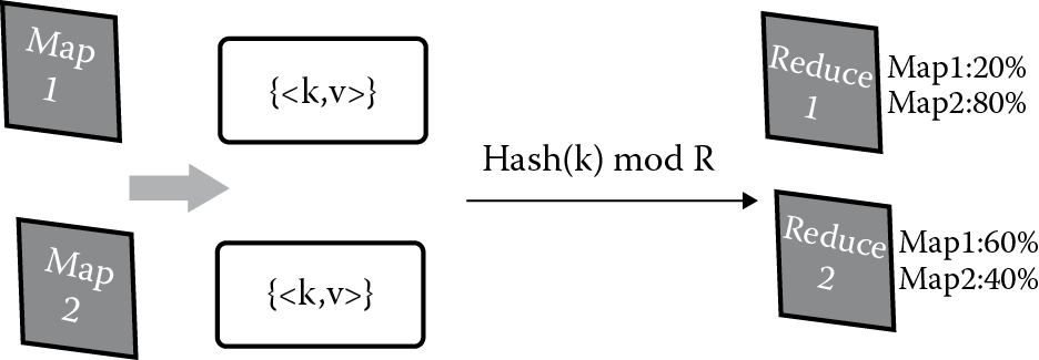
AG—The AG carries out a statistical and predicted test to calculate the distribution of reduce tasks and then start the reduce VM [23] at the appropriate place in the PM. The AG will receive several samples and then will assign its members that contain map and reduce tasks to them. The distribution of intermediate key/value pairs that adopt a hashing approach to distribute the load to the reducers will be computed in reduces.
Placement of reduce virtual machine (VM)—The results of AG will decide the placement of reduce VMs. For example, in Figure 7.5, if 80% of key/value pairs of Reduce1 come from Map2 and the remaining intermediate results are from Map1, the VM of Reduce1 will be started in the physical machine (PM) that contains the VM of Map2. Similarly, the VM of Reduce2 will be started in the PM that includes the VM of Map1.
7.5 NER IN BIOMEDICAL Big Data MINING: A CASE STUDY
Based on the above study of time–space Hadoop MapReduce scheduling algorithms in Sections 7.3 and 7.4, we present a case study in the field of biomedical Big Data mining. Compared to traditional methods and general MapReduce for data mining, our project makes an originally inefficient algorithm become time-bearable in the case of integrating the algorithms in Sections 7.3 and 7.4.
7.5.1 Biomedical Big Data
In the past several years, massive data have been accumulated and stored in different forms, whether in business enterprises, scientific research institutions, or government agencies. But when faced with more and more rapid expansion of the databases, people cannot set out to obtain and understand valuable knowledge within Big Data.
The same situation has happened in the biomedical field. As one of the most concerned areas, especially after the human genome project (HGP), literature in biomedicine has appeared in large numbers, reaching an average of 600,000 or more per year [24]. Meanwhile, the completion of the HGP has produced large human gene sequence data. In addition, with the fast development of science and technology in recent years, more and more large-scale biomedical experiment techniques, which can reveal the law of life activities on the molecular level, must use the Big Data from the entire genome or the entire proteome, which results in a huge amount of biological data. These mass biological data contain a wealth of biological information, including significant gene expression situations and protein–protein interactions. What is more, a disease network, which contains hidden information associated with the disease and gives biomedical scientists the basis of hypothesis generation, is constructed based on disease relationship mining in these biomedical data.
However, the most basic requirements for biomedical Big Data processing are difficult to meet efficiently. For example, key word searching in biomedical Big Data or the Internet can only find lots of relevant file lists, and the accuracy is not high, so that a lot of valuable information contained in the text cannot be directly shown to the people.
7.5.2 Biomedical Text Mining and NER
In order to explore the information and knowledge in biomedical Big Data, people integrate mathematics, computer science, and biology tools, which promote the rapid development of large-scale biomedical text mining. This refers to the biomedical Big Data analysis process of deriving high-quality information that is implicit, previously unknown, and potentially useful from massive biomedical data.
Current research emphasis on large-scale biomedical text mining is mainly composed of two aspects, that is, information extraction and data mining. Specifically, it includes biomedical named entity recognition (Bio-NER), relation extraction, text classification, and an integration framework of the above work.
Bio-NER is the first and an important and critical step in biomedical Big Data mining. It aims to help molecular biologists recognize and classify professional instances and terms, such as protein, DNA, RNA, cell_line, and cell_type. It is meant to locate and classify atomic elements with some special significance in biomedical text into predefined categories. The process of Bio-NER systems is structured as taking an unannotated block of text and then producing an annotated block of text that highlights where the biomedical named entities are [25].
However, because of lots of unique properties in the biomedical area, such as unstable quantity, nonunified naming rules, complex form, the existence of ambiguity, and so on, Bio-NER is not mature enough, especially since it takes much time. Most current Bio-NER systems are based on machine learning, which needs multiple iterative calculations from corpus data. Therefore, it is computationally intensive and seriously increases recognition time, including model training and inference. For example, it takes almost 5 hours for the CRF model training process using the Genia4ER training corpus, which is only about 14 MB [26]. How do we deal with huge amounts of biomedical text data? How do we cope with the unbearable wait for recognition for a very long time? It is natural to seek distributed computing and parallel computing to solve the problem.
7.5.3 MapReduce for CRFs
CRFs are an important milestone in the field of machine learning, put forward in 2001 by John Lafferty et al. [27]. CRFs, a kind of discriminant model and an undirected graph model at the same time, define a single logarithmic linear distribution for a joint probability of an entire label sequence based on a given particular observation sequence. The model is widely used in natural language processing (NLP), including NER, part-of-speech tagging, and so on.
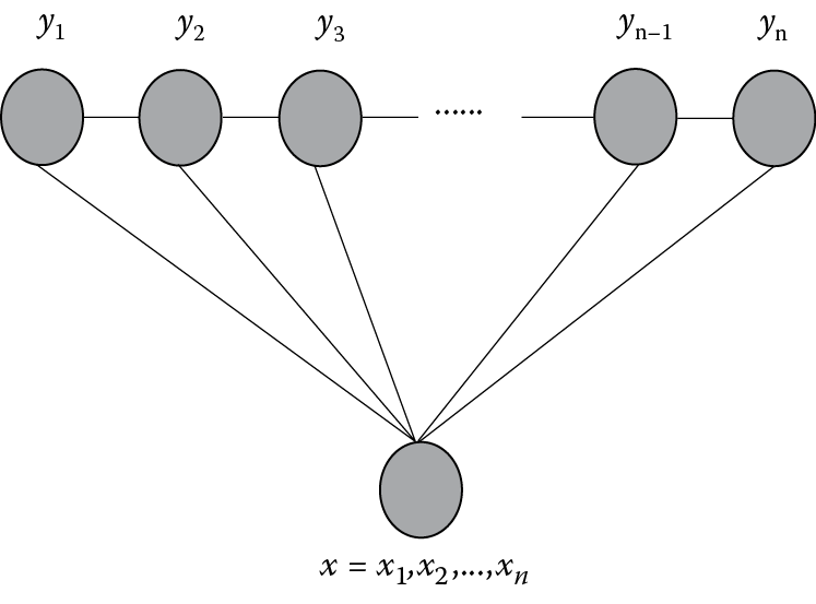
Figure 7.6 shows the CRF model, which computes the conditional probability of an output sequence under the condition of a given input sequence .
A linear CRF, which is used in Bio-NER, is as follows:
, (7.4)
where
, (7.5)
i is the position in the input sequence , λk is a weight of a feature that does not depend on location i, and are feature functions.
For the training process of the CRF model, the main purpose is to seek for the parameter that is most in accordance with the training data . Presume every is independently and identically distributed. The parameter is obtained generally in this way:
. (7.6)
When the log-likelihood function L(λ) reaches the maximum value, the parameter is almost the best. However, to find the parameter to maximize the training data likelihood, there is no closed-form solution. Hence, we adopt parameter estimation, that is, the limited-memory Broyden–Fletcher–Goldfarb–Shanno (L-BFGS) algorithm [28], to find the optimum solution.
To find the parameter to make convex function L(λ) reach the maximum, algorithm L-BFGS makes its gradient vector by iterative computations with initial value λ0 = 0 at first. Research shows that the first step, that is, to calculate ∇Li, which is on behalf of the gradient vector in iteration i, calls for much time. Therefore, we focus on the optimized improvement for it.
Every component in ∇Li is computed as follows:
. (7.7)
It can be linked with every ordered pair within that is mutually independent. So we can calculate the difference between and on each of the input sequences in the training set T and then put the results of all the sequences together. As a result, they can be computed in parallel as shown in Figure 7.7.
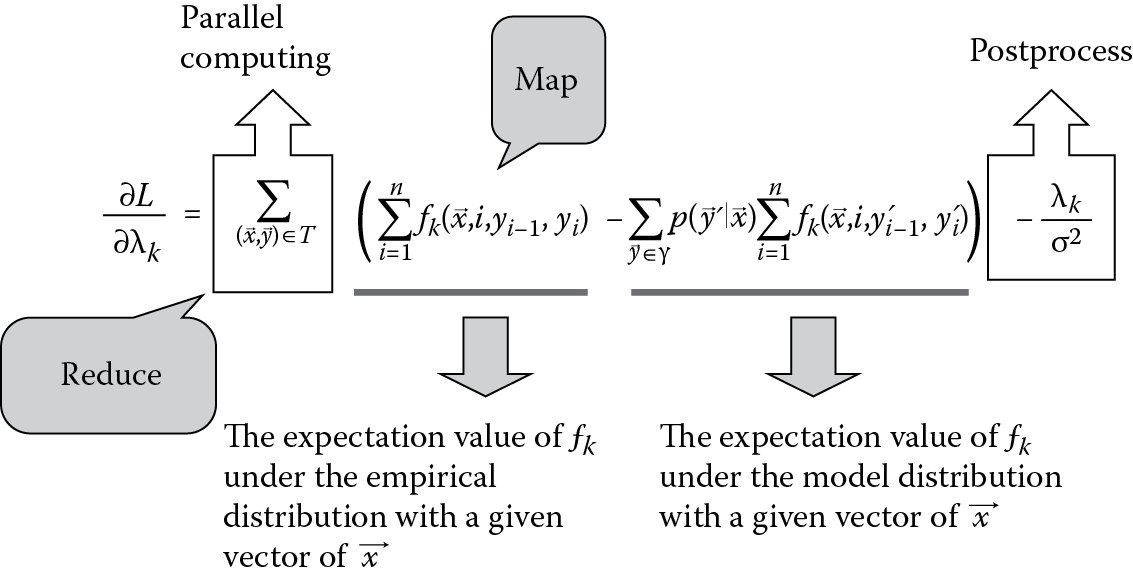
We split the calculation process in-house into several map tasks and summarize the results by a reduce task. And the difference between penalty term is designed to be the postprocessing.
In the actual situation, it is impossible to schedule one map task for one ordered pair because the number of ordered pairs in the large scale of training samples is too huge to estimate effectively. We must syncopate the training data T into several small parts and then start the MapReduce plan as shown in the two above paragraphs at this section.
For a MapReduce Bio-NER application, the data skew leads to uneven load in the whole system. Any specific corpus has its own uneven distribution of the entity (as shown in Table 7.1), resulting in the serious problem of data skew. And protean, artificial defined feature sets exacerbate the problem in both training and inference processes.
Combined with schemes given in this chapter, the uneven load can be solved based on the modified Hadoop MapReduce. The implementation will further improve system performance on MapReduce with time–space scheduling.
7.6 CONCLUDING REMARKS
As data are the basis of information systems, how to process data and extract information becomes one of the hottest topics in today’s information society. This chapter introduces the MapReduce framework, an excellent distributed and parallel computing model. As its implementation, Hadoop plays a more and more important role in a lot of distributed application systems for massive data processing.
For the increasing data and cluster scales, to avoid scheduling delay, scheduling skew, poor system utilization, and low degree of parallelism, this chapter proposes some improved methods that focus on the time and space scheduling of reduce tasks in MapReduce.
Through analyzing the MapReduce scheduling mechanism, this chapter illustrates the reasons for system slot resource wasting that result in reduce tasks waiting around, and it proposes the development of a method detailing the start times of reduce tasks dynamically according to each job context, including the task completion time and the size of the map output. There is no doubt that the use of this method will decrease the reduce completion time and system average response time in Hadoop platforms.
Current Hadoop schedulers often lack data locality consideration. As a result, unnecessary data might get shuffled in the network, causing performance degradation. This chapter addresses several optimizing algorithms to solve the problem of reduce placement. We make a Hadoop reduce task scheduler aware of partitions’ network locations and sizes in order to mitigate network traffic and improve the performance of Hadoop.
Finally, a parallel biomedical data processing model using the MapReduce framework is presented as an application of the proposed methods. As the United States proposed the HGP, biomedical Big Data shows its unique position among the academics. A widely used CRF model and an efficient Hadoop-based method, Bio-NER, have been introduced to explore the information and knowledge under biomedical Big Data.
References
1. J. Tan, S. Meng, X. Meng, L. Zhang. Improving reduce task data locality for sequential MapReduce jobs. International Conference on Computer Communications (INFOCOM), 2013 Proceedings IEEE, April 14–19, 2013, pp. 1627–1635.
2. J. Dean, S. Ghemawat. MapReduce: Simplified data processing on large clusters, Communications of the ACM—50th Anniversary Issue: 1958–2008, 2008, Volume 51, Issue 1, pp. 137–150.
3. X. Gao, Q. Chen, Y. Chen, Q. Sun, Y. Liu, M. Li. A dispatching-rule-based task scheduling policy for MapReduce with multi-type jobs in heterogeneous environments. 2012 7th ChinaGrid Annual Conference (ChinaGrid), September 20–23, 2012, pp. 17–24.
4. J. Xie, F. Meng, H. Wang, H. Pan, J. Cheng, X. Qin. Research on scheduling scheme for Hadoop clusters. Procedia Computer Science, 2013, Volume 18, pp. 2468–2471.
5. Z. Tang, M. Liu, K. Q. Li, Y. Xu. A MapReduce-enabled scientific workflow framework with optimization scheduling algorithm. 2012 13th International Conference on Parallel and Distributed Computing, Applications and Technologies (PDCAT), December 14–16, 2012, pp. 599–604.
6. F. Ahmad, S. Lee, M. Thottethodi, T. N. Vijaykumar. MapReduce with communication overlap (MaRCO). Journal of Parallel and Distributed Computing, 2013, Volume 73, Issue 5, pp. 608–620.
7. M. Lin, L. Zhang, A. Wierman, J. Tan. Joint optimization of overlapping phases in MapReduce. Performance Evaluation, 2013, Volume 70, Issue 10, pp. 720–735.
8. Y. Luo, B. Plale. Hierarchical MapReduce programming model and scheduling algorithms. 12th IEEE/ACM International Symposium on Cluster, Cloud and Grid Computing (CCGRID), May 13–16, 2012, pp. 769–774.
9. H. Mohamed, S. Marchand-Maillet. MRO-MPI: MapReduce overlapping using MPI and an optimized data exchange policy. Parallel Computing, 2013, Volume 39, Issue 12, pp. 851–866.
10. Z. Tang, L. G. Jiang, J. Q. Zhou, K. L. Li, K. Q. Li. A self-adaptive scheduling algorithm for reduce start time. Future Generation Computer Systems, 2014. Available at http://dx.doi.org/10.1016/j.future.2014.08.011.
11. D. Linderman, D. Collins, H. Wang, H. Meng. Merge: A programming model for heterogeneous multi-core systems. ASPLOSXIII Proceedings of the 13th International Conference on Architectural Support for Programming Languages and Operating Systems, March 2008, Volume 36, Issue 1, pp. 287–296.
12. B. Palanisamy, A. Singh, L. Liu, B. Langston. Cura: A cost-optimized model for MapReduce in a cloud. IEEE International Symposium on Parallel and Distributed Processing (IPDPS), IEEE Computer Society, May 20–24, 2013, pp. 1275–1286.
13. L. Ho, J. Wu, P. Liu. Optimal algorithms for cross-rack communication optimization in MapReduce framework. 2011 IEEE International Conference on Cloud Computing (CLOUD), July 4–9, 2011, pp. 420–427.
14. M. Isard, V. Prabhakaran, J. Currey, U. Wieder, K. Talwar, A. Goldberg. Quincy: Fair scheduling for distributed computing clusters. Proceedings of the ACM SIGOPS 22nd Symposium on Operating Systems Principles (SOSP), October 11–14, 2009, pp. 261–276.
15. Wikipedia, Greedy algorithm [EB/OL]. Available at http://en.wikipedia.org/wiki/Greedy_algorithm, September 14, 2013.
16. D. D. Sleator, R. E. Tarjan. Self-adjusting binary search trees. Journal of the ACM (JACM), 1985, Volume 32, Issue 3, pp. 652–686.
17. M. Hammoud, M. F. Sakr. Locality-aware reduce task scheduling for MapReduce. Cloud Computing Technology and Science (CloudCom), 2011 IEEE Third International Conference on, November 29–December 1, 2011, pp. 570–576.
18. S. Huang, J. Huang, J. Dai, T. Xie, B. Huang. The HiBench benchmark suite: Characterization of the MapReduce-based data analysis. Date Engineering Workshops (ICDEW), IEEE 26th International Conference on, March 1–6, 2010, pp. 41–51.
19. M. Hammoud, M. S. Rehman, M. F. Sakr. Center-of-gravity reduce task scheduling to lower MapReduce network traffic. Cloud Computing (CLOUD), IEEE 5th International Conference on, June 24–29, 2012, pp. 49–58.
20. Y. C. Kwon, M. Balazinska, B. Howe, J. Rolia. Skew-resistant parallel processing of feature-extracting scientific user-defined functions. Proceedings of the 1st ACM Symposium on Cloud Computing (SoCC), June 2010, pp. 75–86.
21. P. Dhawalia, S. Kailasam, D. Janakiram. Chisel: A resource savvy approach for handling skew in MapReduce applications. Cloud Computing (CLOUD), IEEE Sixth International Conference on, June 28–July 3, 2013, pp. 652–660.
22. R. Grover, M. J. Carey. Extending Map-Reduce for efficient predicate-based sampling. Data Engineering (ICDE), 2012 IEEE 28th International Conference on, April 1–5, 2012, pp. 486–497.
23. S. Ibrahim, H. Jin, L. Lu, L. Qi, S. Wu, X. Shi. Evaluating MapReduce on virtual machines: The Hadoop case cloud computing. Lecture Notes in Computer Science, 2009, Volume 5931, pp. 519–528.
24. Wikipedia, MEDLINE [EB/OL]. Available at http://en.wikipedia.org/wiki/MEDLINE, September 14, 2013.
25. J. Kim, T. Ohta, Y. Tsuruoka, Y. Tateisi, N. Collier. Introduction to the bio-entity recognition task at JNLPBA. Proceedings of the International Joint Workshop on Natural Language Processing in Biomedicine and Its Applications (JNLPBA), August 2004, pp. 70–75.
26. L. Li, R. Zhou, D. Huang. Two-phase biomedical named entity recognition using CRFs. Computational Biology and Chemistry, 2009, Volume 33, Issue 4, pp. 334–338.
27. J. Lafferty, A. McCallum, F. Pereira. Conditional random fields: Probabilistic models for segmenting and labeling sequence data. Proceedings of the 18th International Conference on Machine Learning (ICML), June 28–July 1, 2001, pp. 282–289.
28. D. Liu, J. Nocedal. On the limited memory BFGS method for large scale optimization. Mathematical Programming, 1989, Volume 45, Issue 1–3, pp. 503–528.