Chapter 5

System Technical Performance Measures

In previous chapters, we have described the systems design processes and some basic models that are utilized within the design process, including the functional analysis and functional allocation models. Models play a significant role in systems design, and rely on variables and parameters to produce valid results. Taking the functional analysis model as an example, for each of the functions in the functional flow block diagram (FFBD), there are performance or constraints parameters that regulate the function to serve the overall system mission. These design-dependent parameters (DDPs) are usually expressed in quantitative format, which are also called technical performance measures (TPMs).

Systems engineering is requirement driven, but, as mentioned before, requirements will not design the system, it is the technical specifications derived from the requirements that will lead to the realization of the system. Based on system requirements, TPMs provide detailed quantitative specifications for system configurations, regulate system technical behavior, and are necessary for designers to obtain the system components, construct the system, and, moreover, to test and evaluate system performance. Developing a precise, accurate, and feasible set of TPMs comprehensively is essential for the mission success of the system design.

In this chapter, we will review some of the most popular system design parameters and the TPMs relevant to them, and describe the fundamental models to analyze and integrate these TPMs into the systems design life cycle. More specifically, we will

1. Provide a comprehensive overview of system DDPs and TPMs and describe their significance for system design and evaluation.
2. Review some commonly used TPMs for systems engineering, including reliability, maintainability, producibility, supportability, usability, and system sustainability. The definitions as well as the characteristics of these parameters are given, and the mathematical modeling for these parameters is reviewed in detail.
3. Life cycle consideration and design integration, and implications for the DDPs, are illustrated so that readers will have guidelines for how these DDPs and TPMs are developed and applied within the various stages of the system life cycle.

On completion of this chapter, readers will have some basic understanding of the general pictures of the technical side of system parameters, know the scope and challenge to develop these parameters, and be familiar with common used analytical models and concepts, so that they may use the right model in the future practice of system design.

5.1 Technical Performance Measures (TPMs)

System technical performance measures, or TPMs, are the quantitative values for the DDPs that describe, estimate or predict the system technical behaviors. TPMs define the attributes for the system to make the system unique so that it can be realized. Examples of TPMs include systems functional parameters (such as size, weight, velocity, power, etc.), system reliability (i.e., mean time between failures [MTBF]), system maintainability (i.e., mean time between maintenance [MTBM]), usability (i.e., human error) and system sustainability.

Table 5.1 illustrates an example for a typical TPM metrics for an automobile. TPMs are derived from requirements analysis; recall that in Section 3.4 on requirement analysis, we discussed the method of using quality function deployment (QFD) to derive and prioritize the TPMs. The development of the TPMs from requirements ensures that the system attributes and behaviors comply with the ultimate users’ needs. TPMs provide estimated quantitative values that describe the system performance requirements. They measure the attributes or characteristics inherent within the design, specifically the DDPs. The identification of TPMs evolves from the development of system operational requirements and the maintenance and support concept. During the system design processes, one of the largest contributors to “risks” is the lack of an adequate system specification in precise quantitative forms. Well-defined TPMs will ensure that (a) the requirements reflect the customers’ needs, and (b) the measurements (metrics) provide designers with the necessary guidance to develop their benchmark.

Another advantage of using TPMs to balance cost, scheduling, and performance specifications throughout the life cycle is to specify measurements of success. Technical performance measurements can be used to compare actual versus planned technical development and design. They also report the degree to which system requirements are met in terms of performance, cost, schedule, and progress in implementation. Performance metrics are traceable to original requirements.

Nevertheless, the types of parameters and TPMs involved in different systems vary a great deal; development of TPMs primarily relies on the clear understanding the nature of the system and the knowledge and experiences of the developers. It is impossible to review every single type of TPM within one chapter, as there is a tremendous amount of information involved in various types of parameter. Specialized models and methods are required to develop specific parameters; for example, physics for the system’s power, acceleration, and velocity. Here, some of the commonly shared parameters are reviewed. These parameters are contained within almost all types of system; they include reliability, maintainability, producibility, supportability, usability, and sustainability. We hope that, by reviewing these basic TPM concepts, readers will gain a comprehensive understanding of the most common parameters that will be involved in the design of most systems, and know how to apply the appropriate methods and models to derive those TPMs accurately. Thus, to that extent, this chapter can be thought of as an extension of Chapter 4, to introduce more systems-design-related models, which are more specific to system DDPs.

5.2 Systems Reliability

5.2.1 Reliability Definition

Generally, system reliability can be defined as follows:

Reliability is the probability that a system or a product will operate properly for a specific period of time in a satisfactory manner under the specified operating conditions. (Blanchard and Fabrycky, 2006)

From the definition, it is easy to see that reliability is a measure of the system’s success in providing its functions properly without failure. System reliability has the following four major characteristics:

1. It is a probability. A system becomes unreliable due to failures that occur randomly, which, in turn, also make system reliability a random variable. The probability of system reliability provides a quantitative measure for such a random phenomenon. For example, a reliability of 0.90 for a system to operate for 80 h implies that the system is expected to function properly for at least 80 h, 90 out of 100 times. A probability measures the odds or the fraction/percentage of the number of times that the system will be functional, not the percentage of the time that the system is working. An intuitive definition of the reliability is as follows: Suppose there are n totally identical components that are simultaneously subjected to a design operating conditions test; during the interval of time [0, t], nf(t) components are found to have failed and the remaining ns(t) survived. At time t, the reliability can be estimated as R(t) = ns(t)/n.
2. Satisfactory performance is specified for system reliability. It defines the criteria at which the system is considered to be functioning properly. These criteria are derived from systems requirement analysis and functional analysis, and must be established to measure reliability. Satisfactory performance may be a particular value to be achieved, or sometimes a fuzzy range, depending on the different types of systems or components involved.
3. System reliability is a function of time. As seen in the definition of system reliability, reliability is defined for a certain system operation time period. If the time period changes, one would expect the value for reliability to change also. It is common sense that one would expect the chance of system failure over an hour to be a lot lower than that over a year! Thus, a system is more reliable for a shorter period of time. Time is one of the most important factors in system reliability; many reliability-related factors are expressed as a time function, such as MTBF.
4. Reliability needs to be considered under the specified operating conditions. These conditions include environmental factors such as the temperature, humidity, vibration, or surrounding locations. These environmental factors specify the normal conditions at which the systems are functional. As mentioned in Chapter 2, almost every system may be considered as an open system as it interacts with the environment regardless, and the environment will have a significant impact on system performance. For example, if you submerge a laptop computer under water, it will probably fail immediately. System reliability has to be considered in the context of the designed environment; it is an inherent system characteristic. System failures should be distinguished from accidents and damage caused by violation of the specified conditions. This is why product warranties do not cover accidents caused by improper use of systems.

The four elements above are essential when defining system reliability. System reliability is an inherent system characteristic; it starts as a design-independent parameter from the user requirements, along with the design process; eventually, reliability will be translated to systems DDPs and TPMs will be derived in specific and quantitative format, so that reliability of the components can be verified. This translation process requires vigorous mathematical models to measure reliability.

5.2.2 Mathematical Formulation of Reliability

5.2.2.1 Reliability Function

As mentioned above, reliability is a function of time, t, which is a random variable denoting the time to failure. The reliability function at time t can be expressed as a cumulative probability, the probability that the system survives at least time t without any failure:

$R\left(t\right)=P(t>t)$ (5.1)

As an assumption for system status, the system is either in a functional condition or a state of failure, so the cumulative probability distribution function of failure F(t) is the complement of R(t), or

$R\left(t\right)+F\left(t\right)=1$ (5.2)

So, knowing the distribution of failure, we can derive the reliability by

$R\left(t\right)=1-F\left(t\right)$ (5.3)

If the probability distribution function (p.d.f., sometimes called probability mass function, p.m.f.) of failure is given by f(t), then the reliability can be expressed as

$R\left(t\right)=1-F\left(t\right)=1-\underset{0}{\overset{t}{{\displaystyle \int }}}f\left(x\right)\text{d}x=\underset{0}{\overset{\infty }{{\displaystyle \int }}}f\left(x\right)\text{d}x-\underset{0}{\overset{t}{{\displaystyle \int }}}f\left(x\right)\text{d}x=\underset{t}{\overset{\infty }{{\displaystyle \int }}}f\left(x\right)\text{d}x$ (5.4)

For example, if the time to failure follows an exponential distribution with parameter λ, then the p.d.f. for failure is

$f\left(t\right)=\lambda e^{-\lambda t}$ (5.5)

The reliability function for time t is

$R\left(t\right)=\underset{t}{\overset{\infty }{{\displaystyle \int }}}\lambda e^{-\lambda x}\text{d}x=e^{-\lambda t}$ (5.6)

One can easily verify Equation 5.6 by using basic integration rules.

5.2.2.2 Failure Rate and Hazard Function

Failure rate is defined in a time interval [t1, t2] as the probability that a failure per unit time occurs in the interval, given that no failure has occurred prior to t1, the beginning of the interval. Thus, the failure rate λ(t) can be formally expressed as (Elsayed 1996)

$\lambda \left(t_2\right)=\frac{{{\displaystyle \int }}_{t_1}^{t_2}f\left(t\right)\text{d}t}{\left(t_2-t_1\right)R\left(t_1\right)}$ (5.7)

From Equation 5.4, it may easily be seen that

$\underset{t_1}{\overset{t_2}{{\displaystyle \int }}}f\left(t\right)\text{d}t=\underset{t_1}{\overset{\infty }{{\displaystyle \int }}}f\left(t\right)\text{d}t-\underset{t_2}{\overset{\infty }{{\displaystyle \int }}}f\left(t\right)\text{d}t=R\left(t_1\right)-R\left(t_2\right)$ (5.8)

So, Equation 5.7 becomes

$\lambda \left(t_2\right)=\frac{R\left(t_1\right)-R\left(t_2\right)}{\left(t_2-t_1\right)R\left(t_1\right)}$ (5.9)

To generalize Equation 5.9, let t1 = t, t2 = t + ∆t, then Equation 5.9 becomes

$\lambda \left(t+\Delta t\right)=\frac{R\left(t\right)-R\left(t+\Delta t\right)}{\nabla t R\left(t\right)}$ (5.10)

The instantaneous failure rate can be obtained by taking the limits from Equation 5.10, as

$\begin{array}{c}\lambda \left(t\right)=\underset{\Delta t\to 0}{\lim }\frac{R\left(t\right)-R\left(t+\Delta t\right)}{\nabla t R\left(t\right)}\\ =\frac{1}{R\left(t\right)}\underset{\Delta t\to 0}{\lim }\frac{R\left(t\right)-R\left(t+\Delta t\right)}{\nabla t }=\frac{1}{R\left(t\right)}\left[-\frac{\text{d}}{\text{d}t}R\left(t\right)\right]\end{array}$ (5.11)

and from Equation 5.4, we have

$\frac{\text{d}}{\text{d}t}R\left(t\right)=-f\left(t\right)$ (5.12)

f(t) is the failure distribution function. So, the instantaneous failure rate is

$\lambda \left(t\right)=\frac{f\left(t\right)}{R\left(t\right)}$ (5.13)

For the exponential failure example, f(t) = λe−λt and R(t) = e−λt, the instantaneous failure rate according to Equation 5.13 is

$\lambda \left(t\right)=\frac{f\left(t\right)}{R\left(t\right)}=\frac{\lambda e^{-\lambda t}}{e^{-\lambda t}}=\lambda$ (5.14)

So, for the exponential failure function, the instantaneous failure rate function is constant over the time. For other types of failure distribution, this might not hold true. For illustration purposes, in this chapter we focus on exponential failure rate function, as exponential failure is commonly found in many applications. For other types of failure functions, one should not assume they have the same characteristics as exponential failure. The specific failure rate function should be derived using Equations 5.10 and 5.11 and the rate is not expected to be constant. Please refer to Appendix I for a comprehensive review for the various distribution functions.

The failure rate λ, generally speaking, is the measure of the number of failures per unit of operation time. The reciprocal of λ is MTBF, denoted as θ:

$\theta =\frac{1}{\lambda }$ (5.15)

Here, we use several examples to illustrate the estimation of the failure rate. As the first example, suppose that one manufacturer of an electric component is interested in estimating the mean life of the component. One hundred components are used for a reliability test. It takes 1000 h for all the 100 components to fail under the specified operating conditions. The components are observed and failures in a 200 h interval are recorded, shown in Table 5.2.

The failure rate for each of the 200 h intervals according to Equation 5.13 is given in Table 5.3.

For a constant failure rate, the failure rate can also be estimated by using the following formula:

$\lambda =\frac{\text{Number of failures}}{\text{Total operating hours}}$ (5.16)

Let us look at another example which is slightly different from the first example. Suppose that one manufacturer of an electric component is interested in estimating the mean life of the component. Ten components are used for a reliability test of 100 h under the specified operating conditions. During the 100 h, seven failures are observed. Table 5.4 lists the occurrence times for all these failures.

So, based on Equation 5.16, the total number of failures for the 100 h is seven, and total operating hours are the sum of all the ten components’ working hours, which is

$15+19+32+45+61+62+89+100+100+100=623$

so the estimation of the failure rate is

$\lambda =\frac{7}{623}=0.01124$

If there is only one component involved and maintenance actions are performed when this component fails so that it is functional again, the failure rate is estimated by the division of the total number of failures over the total time of the component being functional (total time minus downtime). For example, Figure 5.1 shows a component test for a period of 50 h.

So, the total operating hours = 50 − 2.5 − 6.5 − 1.6 − 2.9 = 36.5 h. The failure for this particular component is

$\lambda =\frac{4}{36.5}=0.1096 /\text{h}$

Depending on the different situations in which the test is performed, the appropriate formula should be used to obtain the correct failure rate.

Failure rate, especially instantaneous failure, can be considered as a conditional probability. The failure rate is one of the most important measures for the systems designers, operators, and maintainers, as they can derive the MTBF, or the mean life of components, by taking the reciprocal of the failure rate, expressed in Equation 5.15. MTBF is one common measure for systems reliability due to its simplicity of measurement and its direct relationship to the systems reliability measure.

It is also easily seen that failure rate is a function of time; it varies with different time intervals and different times in the system life cycle. If we plot the system failure rate over time from a system life cycle perspective, it exhibits a so-called “bathtub” curve shape, as illustrated in Figure 5.2.

At the beginning of the system life cycle, the system is being designed, concepts are being explored, and system components are being selected and evaluated. At this stage, because the system is immature, there are many “bugs” that need to be fixed; there are many incompatibilities among components, and many errors are being fixed. The system gradually becomes more reliable along with design effort; thus, the failure rate of the system components decreases. This is the typical behavior of the system failure rate in the early life cycle period, as shown in Figure 5.2 in the first segment of the failure rate curve: the decreasing failure rate period, or the “infant mortality region.”

Once the system is designed and put into operation, the system achieves its steady-state period in terms of failure rate, and presents a relatively constant failure rate behavior. The system is in its maturity period, as presented in the middle region in Figure 5.2. In this stage, system failure is more of a random phenomenon with steady failure rate, which is expected under normal operating conditions.

When the system approaches the end of its life cycle, it is in its wear-out phase, characterized by its incompatibility with new technology and user needs and its worn-out condition caused by its age, it presents a significantly increasing pattern of failure occurrence, as seen in the last region of the life cycle in Figure 5.2. Failures are no longer solely due to randomness but to deterministic factors mentioned above; it is time to retire the system and start designing a new one and a new bathtub curve will evolve again.

Understanding this characteristic of system failure enables us to make feasible plans for preventive and corrective maintenance activities to prolong system operations and make correct decisions about when to build a new system or to fix the existing one.

5.2.2.3 Reliability with Independent Failure Event

Consider a system with n components, and suppose that each component has an independent failure event (i.e., the occurrence of the failure event does not depend on any other; for a more comprehensive review of independent events, please refer to Appendix I at the end of this book). Components may be connected in different structures or networks within the system configuration; these could be in series, in parallel, or a combination thereof.

5.2.2.3.1 Series Structure

Figure 5.3 illustrates a series structure of components. A series system functions if and only if all of its components are functioning. If any one of the components fails, then the system fails; as seen in Figure 5.3, a failed component will cause the whole path to be broken. Here we use a formal mathematical formulation to define the structure functions, so readers may understand the more complex structure better.

Here, we use an indicator variable xi to denote the whether or not the ith component is functioning:

$x_i=\{\begin{array}{l}1,\text{if}i\text{th component is working properly}\hfill \\ 0,\text{if}i\text{th component has failed}\hfill \end{array}$

Thus, the state vector for all the components is ? = (x1,x2,…,xn). Based on the vector, we can define the system structure function as Φ(?) such that

$\Phi \text{(}x)=\{\begin{array}{ll}1, \hfill & \text{if system is working properly when state vector is} x\hfill \\ 0, \hfill & \text{if system has failed when state vector is} x\hfill \end{array}$

So, with a series structure, the structure function is given by

$\Phi \left(x\right)=\min \left(x_1, x_2, \dots , x_n\right)=x_1{x}_2\dots x_n={\displaystyle \prod }_{i=1}^n{x}_i$ (5.17)

From Equation 5.17, it is easily seen that Φ(?) = 1 if and only if all the xi = 1, where i = 1, 2, …, n. So, using the structure function, the reliability of the system consisting of n components in a series structure is given by

$R=\left(R_1\right)\left(R_2\right)\dots \left(R_n\right)$ (5.18)

For example, suppose that a system consists of three components A, B, and C in a series structure, failures occurring in the three components are independent, and the time to failure is exponentially distributed, with λA = 0.002 failure/h, λB = 0.0025 failure/h, and λC = 0.004 failure/h, then the reliability for system ABC for a period of 100 h, according to Equations 5.6 and 5.18, is

$\begin{array}{c}{R}_{ABC}=R_A{R}_B{R}_C=\left(e^{-{\lambda }_{A}t}\right)\left(e^{-{\lambda }_{B}t}\right)\left(e^{-{\lambda }_{C}t}\right)=e^{-({\lambda }_A+{\lambda }_B+{\lambda }_C)t}\\ =e^{-\left(0.002+0.0025+0.004\right)100}=0.4274\end{array}$

If the MTBF is given, then we can use Equation 5.15 to obtain the failure rate by λ = 1/MTBF, and Equation 5.18 can be used to obtain the reliability.

5.2.2.3.2 Parallel Structure

Figure 5.4 presents a structure of components in parallel.

With a parallel structure, a system fails if and only if all the components fail, or, in other words, a parallel system is functioning if at least one component is functioning. So, for all the components xi, if at least one xi = 1, then Φ(?) = 1. Using the same indicator variable and structure function, the structure function of a parallel structure is given by

$\Phi \left(x\right)=\max \left(x_1, x_2, \dots , x_n\right)=1-{\displaystyle \prod }_{i=1}^n\left(1-x_i\right)$ (5.19)

When n = 2, this yields

$\max \left(x_1, x_2\right)=1-\left(1-x_1\right)\left(1-x_2\right)=x_1+x_2-x_1{x}_2$

So, similarly, the reliability function of a parallel system structure is given by

$R=1-\left(1-R_1\right)\left(1-R_2\right)\dots \left(1-R_n\right)$ (5.20)

As an example, suppose that a system consists of three components A, B, and C in a parallel structure, failures occurring in the three components are independent, and the time to failure is exponentially distributed with λA = 0.002 failure/h, λB = 0.0025 failure/h and λC = 0.004 failure/h, then the reliability for system ABC for a period of 100 h is

$\begin{array}{c}{R}_{ABC}=1-(1-R_A)\left(1-R_B\right)\left(1-R_C\right)=1-\left(1-e^{-{\lambda }_{A}t}\right)\left(1-e^{-{\lambda }_{B}t}\right)\left(1-e^{-{\lambda }_{C}t}\right)\\ =1-\left(1-e^{-0.002\left(100\right)}\right)\left(1-e^{-0.0025\left(100\right)}\right)\left(1-e^{-0.004\left(100\right)}\right)=0.9868\end{array}$

Some readers may have noticed that with the same components, the parallel structure has a better reliability (0.9868 vs. 0.4274). If we look at the reliability of each component, $R_A=e^{-{\lambda }_{A}t}=e^{-0.002\left(100\right)}=0.\text{8187}$ , $R_B=e^{-{\lambda }_{B}t}=e^{-0.0025\left(100\right)}=0.\text{7788}$ , and $R_C=e^{-{\lambda }_{C}t}=e^{-0.004\left(100\right)}=0.\text{67}0\text{3}$ , it is obvious that the reliability for the series structure is lower than that of any individual component while the reliability of the parallel structure is higher than that of any individual component. One can prove this proposition easily, since the reliability 0 ≤ R ≤ 1. As a matter of fact, the more components we have in the series structure, the less reliable the system is, and the more components we add to a parallel system, the more reliable it is.

5.2.2.3.3 k-out-of-n Structure and Combined Network

A k-out-of-n system is functioning if and only if at least k components of the n total components are functioning. Recall that we defined xi as a binary function, with xi = 1 if the ith component is working, and xi = 0 otherwise. So, the number of working components for the system can be obtained by ${\sum }_{i=1}^n{x}_i$ . Therefore, the k-out-of-n system structure function Φ(?) can be expressed as

$\Phi \left(x\right)=\{\begin{array}{cc}1, & {\displaystyle \sum _{i=1}^n{x}_i} \ge k\\ 0,& {\displaystyle \sum _{i=1}^n{x}_i}<k\end{array}$ (5.21)

It is easy to see that series and parallel systems are both special cases for the k-out-of-n structure. The series structure is an n-out-of-n system and the parallel structure is a 1-out-of-n system.

Let us look at the following example: Consider a system consisting of five components, and suppose that the system is functioning if and only if components 1, 2, and 3 all function and at least one of the components 4 and 5 functions. This implies that 1, 2, and 3 are in a series structure and 4 and 5 are placed in a parallel structure. So, the structure function for this particular system is

$\Phi \left(x\right)=\min \left(x_1, x_2, x_3\right)\max \left(x_4, x_5\right)=x_1{x}_2{x}_3\left(x_4+x_5-x_4{x}_5\right)$

From the k-out-of-n structure function, one can easily derive the reliability for the k-out-of-n system,

$R_n=P\left\{\Phi \left(x\right)=1\right\}=P\left\{{\displaystyle \sum _{i=1}^n{x}_i}\ge k\right\}$ (5.22)

As an example, for a 2-out-of-4 system, the reliability is given by

$\begin{array}{c}{R}_4=P\left\{\Phi \left(x\right)=1\right\}=P\left\{{\displaystyle \sum }_{i=1}^4{x}_i\ge 2\right\}\\ =P\left\{x=\left(1,1,1,1\right)\right\}+P\left\{x=\left(1,1,1,0\right)\right\}+P\left\{x=\left(1,1,0,1\right)\right\}\\ +P\left\{x=\left(1,0,1,1\right)\right\}+P\left\{x=\left(0,1,1,1\right)\right\}+P\left\{x=\left(1,1,0,0\right)\right\}\\ +P\left\{x=\left(1,0,1,0\right)\right\}+P\left\{x=\left(0,1,1,0\right)\right\}\\ +P\left\{x=\left(1,0,0,1\right)\right\}+P\left\{x=\left(0,1,0,1\right)\right\}+P\left\{x=\left(0,0,1,1\right)\right\}\\ =R_1{R}_2{R}_3{R}_4+R_1{R}_2{R}_3\left(1-R_4\right)+R_1{R}_2(1-R_3)R_4+R_1(1-R_2)R_3{R}_4 \\ +\left(1-\left(1-R_1\right)R_2{R}_3{R}_4+R_1{R}_2(1-R_3\right)\left(1-R_4\right)+R_1(1-R_2)R_3\left(1-R_4\right)\\ +(1-R_1)R_2{R}_3\left(1-R_4\right)+R_1(1-R_2)\left(1-R_3\right)R_4\\ +(1-R_1)R_2(1-R_3)R_4+(1-R_1)(1-R_2)R_3{R}_4\end{array}$

If all the components are identical, with the same probability of R, Equation 5.22 is given by

$R_n=P\left\{\Phi \left(x\right)=1\right\}=P\left\{{\displaystyle \sum }_{i=1}^n{x}_i\ge k\right\}={\displaystyle \sum }_{i=k}^n\left(\begin{array}{c}n\\ i\end{array}\right)R^i{\left(1-R\right)}^{n-i}$ (5.23)

$\left(\begin{array}{c}n\\ i\end{array}\right)$ is a k-combination function, measuring the number of subsets of k elements taken from a set of n elements (n ≥ k).

$\left(\begin{array}{c}n\\ i\end{array}\right)=\frac{n\left(n-1\right)\dots \left(n-i+1\right)}{i\left(i-1\right)\dots 1}=\frac{n!}{i!\left(n-i\right)!}$

Using the concepts above, one can easily solve the reliability for any combined network consisting of series and parallel structures. Let us look at one example: Suppose that a system consists of five components, A, B, C, D, and E, they are connected in the structure shown in Figure 5.5.

Assuming the failure functions for A, B, C, D, and E are exponentially distributed and the MTBFs for these components are shown as follows:

${\text{MTBF}}_A=10,000 \text{h}$

${\text{MTBF}}_B=8000 \text{h}$

${\text{MTBF}}_C=5000 \text{h}$

${\text{MTBF}}_D=2500 \text{h}$

${\text{MTBF}}_E=20,000 \text{h}$

What is the probability of the system ABCDE surviving for 5000 h without failure?

From Figure 5.5, we can see that components A and B are in a series structure; A/B, C, and D are connected in a parallel structure; and, finally, ABCD are connected with E in a series structure. The failure rates for these components are

${\lambda }_A=\frac{1}{10,000}=0.0001 \text{failure/h}$

${\lambda }_B=\frac{1}{8000}=0.000125 \text{failure/h}$

${\lambda }_C=\frac{1}{5000}=0.0002 \text{failure/h}$

${\lambda }_D=\frac{1}{2500}=0.0004 \text{failure/h}$

${\lambda }_E=\frac{1}{20,000}=0.00005 \text{failure/h}$

The reliability for A and B is

$\begin{array}{c}{R}_{AB}=R_A{R}_B=\left(e^{-{\lambda }_{A}t}\right)\left(e^{-{\lambda }_{B}t}\right)=e^{-\left({\lambda }_A+{\lambda }_B\right)t}\\ =e^{-\left(0.0001+0.000125\right)5000}=0.32465\end{array}$

because

$R_C=e^{-\left({\lambda }_C\right)t}=e^{-\left(0.0002\right)5000}=0.36788$

$R_D=e^{-\left({\lambda }_D\right)t}=e^{-\left(0.0004\right)5000}=0.13536$

The composite reliability for ABCD is

$\begin{array}{c}{R}_{ABCD}=1-\left(1-R_{AB}\right)\left(1-R_C\right)\left(1-R_D\right)\\ =1-\left(1-0.32465\right)\left(1-0.36788\right)\left(1-0.13536\right)=0.63088\end{array}$

since

$R_E=e^{-\left({\lambda }_E\right)t}=e^{-\left(0.00005\right)5000}=0.7788$

So, the reliability for the overall system ABCDE is given by

$R_{ABCDE}=R_{ABCD}{R}_E=\left(0.63088\right)\left(0.7788\right)=0.4913$

This implies that the probability of the system ABCDE surviving for an operating time of 5000 h is about 49.13%, or the system reliability for 5000 h is 49.13%. For a number of operating hours less than 5000, one would expect this reliability to increase.

From the above example, we can see that the general procedure for solving a system reliability problem is quite simple and straightforward; no matter how complex the system structure is, it can always be decomposed into one of the two fundamental structures, series and parallel. So, one would follow these steps:

1. Obtain the reliability value for the individual components for the time t.
2. Start from the most basic structure, and gradually work up to the next level, until the whole system structure is covered. For the above example, we started with the bottom level of the structure, which is A and B, obtaining the reliability of RAB, so A and B may be treated as being equivalent to one component in terms of reliability; then, we address A/B, C and D; they are the next level’s basic structure, as they are a three-branched parallel structure; and finally we obtain the system reliability as the overall structure is a large series network between A/B/C/D and E.

Using the above two procedures, one can easily obtain reliability measures for any complex network structures. There are some exercise questions at the end of the chapter; readers may practice applying these procedures and formulas.

The reliability examples we have talked about so far have only considered the case when the first failure occurs; there are certain circumstances in which components can be replaced when one component fails. To simplify the situation, let us assume the replacement happens immediately (i.e., time to replace = 0), or we can imagine a redundant system design: When one component fails, there is a switch to connect a backup component instantly, as shown in Figure 5.6. This type of system is also called a redundant standby network.

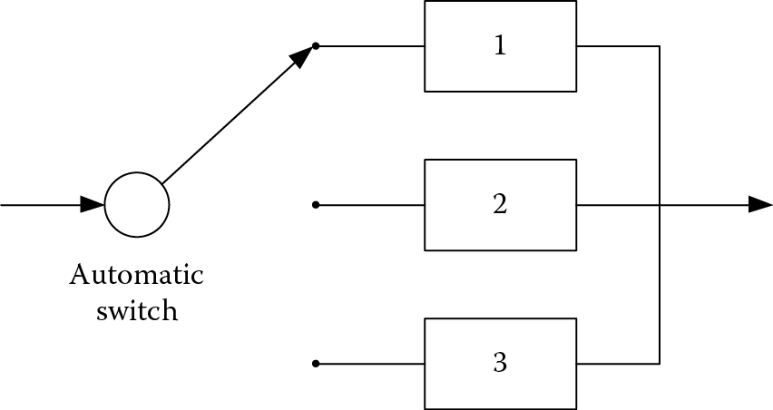
In a standby system, the backup component is not put into operation until the preceding component fails. For example, in Figure 5.6, at the beginning, only Component 1 is operative while Components 2 and 3 are standing by. When Component 1 fails, Component 2 is immediately put in use until it fails; then, Component 3 becomes operational. When Component 3 fails, the system stops working and this is considered a system failure.

In standby systems, the failures of individual components are not totally independent of each other; this is different from a purely parallel network, in which failures occur independently. In standby structures, failures occur one at a time, while in the parallel network, two parts can fail at the same time.

Assuming that the failure function is still exponential (i.e., the time to fail follows an exponential distribution), to simplify the situation, let us further assume that all the parts are identical. The failures occur one by one, so for an N-component standby system, the system is functional until N failures occur. Put in a formal way, if we denote the random variable ℕt as the number of failure occurring in time t, then we have

$R\left(n \text{standby}\right)=P\left({\mathbb{N}}_t\le N\right)$ (5.24)

It is known that when the interval time between failures follows an exponential distribution with parameter λ, then the probability distribution of the number of failures occurring in any time interval of t follows a Poisson distribution with parameter λt. The Poisson distribution can be defined as follows:

A discrete random variable ℕ has a Poisson distribution with parameter λ if for n = 0, 1, 2, …

$P\left(\mathbb{N}=n\right)=\frac{e^{-\lambda }{\lambda }^n}{n!}$ (5.25)

So, the number of failures occurring during any time interval t is given by the following formula:

$P\left({\mathbb{N}}_t=n\right)=\frac{e^{-\lambda t}\lambda t^n}{n!}$

The reliability for the standby system can be written as

$R\left(N\text{standby}\right)=P\left({\mathbb{N}}_t\le N\right)={\displaystyle \sum }_{n=0}^N\frac{e^{-\lambda t}\lambda t^n}{n!}$ (5.26)

As an example, suppose that a system consists of one component with two other identical ones (three components in total) in standby. Each of the components has an MTBF of 2500 h, distributed exponentially. Determine the system reliability for a period of 100 h.

$\lambda =\frac{1}{2500}=0.0004 \text{failures}\text{}/\text{h}$

$\lambda t=0.0004\left(100\right)=0.04 \text{failures}$

Based on Equation 5.26, the system reliability is

$\begin{array}{c}R\left(2\text{standby}\right)=P\left({\mathbb{N}}_t\le 2\right)\\ =e^{-0.04}+\left(0.04\right)e^{-0.04}+\frac{{\left(0.04\right)}^2{e}^{-0.04}}{2!}=0.99997\end{array}$

If these three components are configured in a parallel structure, then the reliability is

$R\left(3\text{parallel}\right)=1-{\left(1-e^{-0.04}\right)}^3=0.99994$

which is less than 0.99997. A standby structure provides higher reliability than a parallel structure with the same components. This may be easily seen, as the reliability is a function of time; the standby system uses one part after another fails, so all the parts except the first one have a later start time than parts in a parallel structure. Thus, it is anticipated that those parts in standby systems will last longer.

There are many other situations that can also be modeled as a standby system. For example, when one component fails, it can be replaced by a backup component from the inventory so that the system still functions. If the replacement time is relatively short enough to be ignored, then the reliability of the system can be approximated by treating it as a standby structure. Or, in other words, if we look at all the components together as a whole system, it is as if the overall system MTBF has been prolonged; that is, for an N-component standby system, if each of the components has a failure rate of λ, then the overall system MTBF = N(MTBF) = N/λ, so the system failure rate λN = λ/N. However, we cannot use Equation 5.6 to obtain the reliability of the system, because the failure function for the system is no longer exponentially distributed.

5.2.3 Reliability Analysis Tools: FMEA and Faulty Trees

System reliability, as one of the inherent design characteristics, is one of the most important parts of any system’s operational requirements, regardless of what type of system it is. Starting from a very high level, requirements regarding system reliability are defined both quantitatively and qualitatively, including

1. Performance and effectiveness factors for system reliability
2. System operational life cycle for measuring reliability
3. Environmental conditions in which the system is expected to be used and maintained (such as temperature, humidity, vibration, radiation, etc.)

The original requirements are derived from users, mission planning, and feasibility analysis. Once the high-level requirements are obtained, lower-level requirements are developed as the system design evolves; system requirements need to be allocated to the system components. System reliability is allocated in the system TPMs and integrated within the functional analysis and functional allocation processes.

When allocating to the lower levels of the system, there is, unfortunately, no template or standard to follow, as every system is different and there may be tens of thousands of parts involved in multiple levels. Most of the allocations utilize a trial-evaluation-modify cycle until a feasible solution is reached. This approach uses a bottom-up procedure as well the top-down process, as different COTS components are considered for selection. Under these circumstances, it is very difficult to arrive at optimum solutions; usually a feasible solution meeting the system requirements and complying with all other design constraints is pursued, and this process is also iterative and often involves users.

Throughout the design, as part of the iterative design and evaluation process, there are many analysis tools that are available to aid the designers to effectively derive the requirements and TPMs for system reliability at different levels of the system structure. For most systems, the reliability requirements are addressed in an empirical manner; with a large volume of requirements and many iterations of analysis-integration-evaluation, one needs to have a practical tool to elicit the structures and relationships required for system reliability, so that the TPMs can be determined. Two of the most commonly used tools are failure mode effect analysis (FMEA) and faulty tree analysis (FTA).

5.2.3.1 Failure Mode Effect Analysis (FMEA)

Failure mode effect analysis (FMEA), sometimes called failure mode, effects, and criticality analysis (FMECA), is a commonly used analysis tool for analyzing failures that are associated with system components. It was originally developed by NASA to improve the reliability of hardware design for space programs. Although the original FMEA document is no longer in effect, the FMEA methodology, however, has been well preserved and tested and has evolved. Nowadays, FMEA has become a well-accepted standard for identifying reliability problems in almost any type of systems, ranging from military to domestic and mechanical to computer software design.

Generally speaking, FMEA is a bottom-up inductive approach to analyze the possible component failure modes within the system, classifying them into different categories, severities, and likelihoods, identifying the consequences caused by these failures to develop a proactive approach to prevent them from occurring, and the related maintenance policy for these failures. It is an inductive process, because FMEA starts with detailed specific examples and cases of failure, to gradually derive general propositions regarding system reliability predictions (as opposed to the deductive approach, where the specific examples are derived from the general propositions, as in the faulty tree analysis approach we will discuss in Section 5.2.3.2).

FMEA usually consists of two related but separate analyses; one is FMEA, which investigates the possible failure modes at different system levels (components or subsystems) and their effects on the system if failure occurs; the second is criticality analysis (CA), which quantifies the likelihood of failure occurrence (i.e., failure rate) and ranks the severity of the effects caused by the failures. This ranking is usually accomplished by analyzing historical failure data from similar systems/components and through a team approach, derived in a subjective manner.

To conduct an FMEA analysis, there are some basic requirements that need to be fulfilled first. These requirements include:

1. System structure in schematic form. Without the basic understanding of the system architecture, especially the hardware and software structures, one cannot identify the possible consequences if one or more components fail. This is the starting point of FMEA analysis.
2. System function FFBD. As we stated earlier, the FFBD is the foundation for many analyses; only with the FFBD specified, functions can then be allocated to components, components allocated to hardware, software or humans, and the operational relationships between the components defined, which is necessary to conduct FMEA analysis.
3. Knowledge of systems requirements. System hardware and software architecture is derived based on requirements. At any point in the design, requirements are needed to verify the design decisions; ultimately, this is important for FMEA-related analysis, since FMEA is an inductive approach and everything is assessed on an empirical basis.
4. A comprehensive understanding of the systems components. This includes, but is not limited to, access to current technology, understanding of the COTS items, and knowledge of supply chain operations and structures related to system components.

With the basic sources of information available and preliminary assessment of the system structure, a team approach is applied to develop the FMEA analysis results; the basic steps are illustrated in Figure 5.7.

1. Define system requirements. Requirements for system reliability need to be clearly defined, as do the TPMs (such as the MTBF of the system) and the system operating environments. With high-level systems requirements defined and refined at a lower level, the system structures can be identified, via a top-down approach, from system to subsystem level, down to the components and eventually the hardware and software units to construct the systems. This provides a big picture for system reliability and a starting point to conduct FMEA analysis.
2. Construct system FFBD. One thing we have to keep in mind is that FMEA analysis has be based on the system design synthesis and integration results. Ideally, FMEA analysis should be paired with system functional analysis and functional allocation, as FMEA analysis is tied to each system component. To perform an FMEA analysis, the following materials/information are needed from functional analysis:
   1. System functional architecture and mission requirements.
   2. System FFBD.
   3. System operational information for each of the functions, similarly to Figure 4.10; input/output, mechanism, and constraints information are required to identify the failure mode and its effects.
   4. Rules, assumptions, and standards pertaining to components. Understanding the limitations of the current feasible technology and COTS constraints helps us to make predictions of the failure mode more meaningful. The ground rules generally include system mission, phase of the mission, operating time and cycle, derivation of failure mode data (i.e., supplier data, historical log, statistical analysis, subject matter experts’ estimates, etc.), and any possible failure detection concepts and methodologies.
3. Requirements allocation and function allocation: With the FFBD, the reliability-related TPMs are allocated to the components level; this is parallel to the function allocation process, described in Section 4.3.2. With the requirements allocated to the lower levels, the effects of failure on the system can be specified at a quantitative level.
4. Identify failure mode. A failure mode is the manner in which a failure occurs at a system, subsystem, or component level. There are many types of failure mode involved in a single component; to derive a comprehensive analysis of the failure mode, designers should look at the various sources of information, including similar systems, supplier data, historical data for critical incidents and accidents studies, and any information related to environmental impacts. A typical component failure mode should include the following aspects:
   1. Failure to operate in proper time
   2. Intermittent operation
   3. Failure to stop operating at the proper time
   4. Loss of output
   5. Degraded output or reduced operational capability
5. Identify causes and effects of failure. The cause of the failure mode is usually an internal process or external influence, or an interaction between these. It is very possible that more than one failure could be caused by one process and a particular type of failure could have multiple causes. Typical causes of a failure include aging and natural wearing out of the materials, defective materials, human error, violation of procedures, damaged components due to environmental effects, and damage due to the storage, handling, and transportation of the system. There are many tools to aid designers in laying out the sources and effects of failures and their relationships; for example, the “fishbone” diagram by Ishikawa, the Swiss model, and the human factors analysis and classification system (HFACS) for human error analysis have been widely used to identify the complex structure of error cause–effect relationships. Failure effect analysis assesses the potential impact of a failure on the components or the overall system. Failures impact systems at different levels, depending on the types of failures and their influences. Generally speaking, there are three levels of failure effect:
   1. Local effect: Local effects are those effects that result specifically from the failure mode of the component at the lowest level of the structure itself.
   2. Parent-level effect: These are the effects that a failure has on the operation and performance of the functions at the immediate next higher level.
   3. End-level effect. These effects are the ones that impact on the operation and functions on the overall system as a whole. A small failure could cause no immediate effect on the system for a short period of time, cause degraded system overall performance, or cause the system to fail with catastrophic effects.
6. Identify failure detection method. This section of FMEA identifies the methods by which the occurrence of a failure is detected. These methods include
   1. Human operators
   2. Warning devices (visual or auditory)
   3. Automatic sensing devices

   The detection methods should include the conditions of detection (i.e., normal vs. abnormal system operations) and the times and frequencies of the detection (i.e., periodic maintenance checking to identify signs of potential failure, or diagnosis of failure when symptoms are observed).

7. Assign failure severity. After all failure modes and their effects on the system are identified, the level of impact of these failures on the system need to be ranked by assigning an appropriate severity score. This will enable design teams to prioritize failures based on the “seriousness” of the effect, so that they can be addressed in a very efficient way, especially given the limited resources available. To assign a severity score for each of the failure modes, each failure effect is evaluated in terms of the worst consequences of the failure on the higher-level system, and through iterative team efforts, a quantitative score is assigned to that particular failure. Table 5.5 illustrates a typical severity ranking and scales.
8. Assign failure mode frequency and probability of detection. This is the start of the second half of the FMEA analysis, the criticality analysis (CA). It adds additional information about the system failure so that a better design can be achieved by avoiding these failures. The CA part of FMEA enables designers to identify the system reliability- and maintainability-related concerns and address these concerns in the design phase. The first step of CA is to transfer the data collected to determine the failure rate; that is, the frequency of failure occurrence. This rate is often expressed as a probability distribution as the failure occurs in a random manner. It also includes the information about the accuracy of failure detection methods, combining the probability of failure detection (i.e., a correct hit detection, or a false alarm detection) to provide the level of uncertainty of failure occurrence and the probability of the failure being detected.
9. Analyze failure criticality. Once the failure rate and detection probability of the failure has been identified, information pertaining to the failure needs to be consolidated to form a criticality assessment of the failure for it to be addressed in the design. Criticality can be assessed quantitatively or qualitatively. For a quantitative assessment, various means or measures can be used to calculate the critical values of the components; for example, the required number of backup (redundant) parts for a predetermined reliability level, as expressed in Equation 5.26, identifying the item criticality score (Cm) for each of the items. If the failure rate is λ, the failure mode probability is α, and the failure effect probability is β, then the failure mode criticality score for a time period of t is given by

$C_m\left(t\right)=\alpha \beta \lambda t$ (5.27)

If the item has a number of different failure modes, then the item criticality number is the sum of all the failure mode criticality numbers, given by

$C_y\left(\text{t}\right)={{\displaystyle \sum }}^{\text{}}{C}_{mi}\left(\text{t}\right)={{\displaystyle \sum }}^{\text{}}{\alpha }_i{\beta }_i{\lambda }_i\text{t}$ (5.28)

Qualitative analysis is used when the failure rate for the item is not available. A typical method used in qualitative analysis is to use the risk priority number (RPN) to rank and identify concerns or risks associated with the components due to the design decisions. The number provides a mean to delineate the more critical aspects of the systems design. The RPN can be determined from:

RPN = (severity rating) × (frequency rating) × (probability of detection rating)

Generally speaking, a component with a high frequency of failure, high impact/severity of failure effect, and difficulty of failure detection usually has a high RPN. Such components should be given high priority in the design consideration.

It is convenient to present a finished FMEA analysis in a tabular format, listing all the required information in different columns. Table 5.6 presents a sample set of FMEA analysis results an automobile.

5.2.3.2 Faulty Tree Analysis (FTA)

A faulty tree analysis, or FTA model, is a graphical method for identifying the different ways in which a particular component/system failure could occur. Compared to the FMEA model, which is considered a “bottom-up” inductive approach, FTA is a deductive approach, using graphical symbols and block diagrams to determine the events and the likelihood (probability) of an undesired failure event occurring. FTA is used widely in reliability analysis where the cause–effect relationships between different events are identified. Figure 5.8 illustrates the basic symbols that an FTA model uses.

FTA models are usually paralleled with functional analysis, providing a concise and orderly description of the different possible events and the combination thereof that could lead to a system/subsystem failure. FTA is commonly used as a design method, based on the analysis of similar systems and historical data, to predict causal relationships in terms of failure occurrences for a particular system configuration. The results of FTA are particularly beneficial for designers to identify any risks involved in the design, and more specifically to

1. Allocate failure probabilities among lower levels of system components
2. Compare different design alternatives in terms of reliability and risks
3. Identify the critical paths for system failure occurrence and provide implications of avoiding certain failures
4. Help to improve system maintenance policy for more efficient performance

Generally speaking, there are four basic steps involved in conducting an FTA analysis:

Step 1: Develop the functional reliability diagram. Develop a functional block diagram for systems reliability, based on the system FFBD model, focusing on the no-go functions and functions of diagnosis and detection. Starting from the system FFBD, following the top-down approach, a tree structure for critical system failure events is identified. This diagram includes information about the structures of the no-go events, what triggers/activates the events, and what the likelihoods and possible consequences of those events are.

Step 2: Construct the faulty tree. Based on the relationships described in the functional diagram, a faulty tree is constructed by using the symbols from Figure 5.8. The faulty tree is based on the functional diagram but is not exactly the same, in the sense that functional models follow the system operational sequences of functions while the FTA tree follows the logical paths of cause–effect failure relationships; it is very possible that, for different operational modes, multiple FTAs may be developed for a single functional path. In constructing the faulty tree, the focus is on the sequence of the failure events for a specific functional scenario or mission profile.

Step 3. Develop the failure probability model. After the FTA is constructed, the next step is to quantify the likelihood of failure occurrence by developing the probability model of the faulty tree. Just as in understanding the models of reliability theory, readers need to familiarize themselves with basic probability and statistics theory. The fundamentals of probability and statistics are reviewed in Appendix I at the end of this book; readers must first engross themselves in these subjects to understand these models. As a matter of fact, in terms of quantitative modeling methodology for systems engineering, probability and statistics are perhaps the most important subjects besides operations research; due to the uncertain and dynamic nature of complex system design, one can hardly find any meaningful solution to a system design problem without addressing its statistical nature. We will be covering more on this subject in later chapters and Appendix I.

The mathematical model of FTA is primarily concerned with predicting the probability of an output failure event with the probabilities of events that cause this output failure. For simplification purposes, we assume all the input failures are independent of each other. Two basic constructs for predicting the output events are the AND-gate and the OR-gate.

5.2.3.2.1 AND-gate

All the input events (Ei, i = 1, 2, …, n) attached to the AND-gate must occur in order for the output event (A) above the gate to occur. That is to say, in terms of the probability model, the output event is the intersection of all the input events. For example, for the AND-gate illustrated in Figure 5.9, if we know the probability of the input events as P1, P2, …, Pn, the probability of output failure above the AND-gate can be obtained as P(A)=P(E1∩E2∩…∩En). Since all the input events are independent of each other, P(A) is the product of all the input event probabilities, that is, P(A) = P1P2…Pn.

For example, for a three-branched AND-gate as illustrated in Figure 5.10,

if P1 = 0.95, P2 = 0.90, and P3 = 0.92, then

$P\left(A\right)=P_1{P}_2{P}_3=\left(0.95\right)\left(0.90\right)\left(0.92\right)=0.79$

5.2.3.2.1 OR-gate

If a failure occurs if one or more of the input events (Ei, i = 1, 2, …, n) occurs, then an OR-gate is used for this causal relationship. In terms of the probability model, the OR-gate structure represents the union of the input events attached to it. For example, for the OR-gate illustrated in Figure 5.11, if we know the probability of the input events as P1, P2,…, Pn, the probability of output failure above the OR-gate can be obtained as $P\left(O\right)=P\left(E_1\cup E_2\cup \dots \cup E_n\right)$ . Since all the events are not mutually exclusive, we cannot simply use the sum of the probability of the events. To solve for P(O), we need to use the concept of the compliment, that is, $P\left(O\right)=1-P\left(\overline{O}\right)$ , $P\left(\overline{O}\right)$ is the probability that none of the input events occurs; this means that all the events must not occur together. So we have $P\left(\overline{O}\right)=P\left(\overline{E_1}\cap \overline{E_2}\cap \dots \cap \overline{E_n}\right)$ ; thus we can obtain P(O) by $P\left(O\right)=1- P\left(\overline{E_1}\cap \overline{E_2}\cap \dots \cap \overline{E_n}\right)=1-\left(1-P_1\right)\left(1-P_2\right)\dots \left(1-P_n\right)$ , or

$P\left(O\right)=1-{\displaystyle \prod }_{i=1}^n\left(1-P_i\right), i=1,2, \dots ,n$

For example, for a three-event OR-gate, as illustrated in Figure 5.12, if P4 = 0.95, P5 = 0.90, and P6 = 0.92, then

$\begin{array}{c}P\left(B\right)=1-\left(1-P_4\right)\left(1-P_5\right)\left(1-P_6\right)\\ =1-\left(1-0.95\right)\left(1-0.90\right)\left(1-0.92\right)=0.9996\end{array}$

After talking about AND-gates and OR-gates, some readers may easily see that the calculation of the AND-gate is similar to the series structure and the OR-gate is similar to the parallel structure of the reliability network. This is because the logic for the AND and OR of failure events are the same as the reliability events in the series and parallel structures. Understanding the basic probability model for the AND-gate and OR-gate, we can solve any composite faulty tree structure; we just start from the bottom level and work our way up, until the probabilities for all the events are obtained. Take the example of the FTA in Figure 5.13. If we know P1 = 0.60, P2 = 0.75, P3 =0.90, P4 =0.95, and P5 = 0.80, what is the value of P(C)?

First, Event A is an OR-gate from Event 1/Event 2, so P(A) = 1 − (1−P1)(1−P2) = 1−(0.40)(0.25) = 0.90; next, Event B is an AND-gate from Event 3/Event 4, so P(B) = P3P4 = (0.90)(0.95) = 0.855; and finally, C is a an OR-gate event from Event A/Event B/Event 5, so P(C) = 1−[1−P(A)][1−P(B)][1−P5] = 1−(1−0.90)(1−0.855)(1−0.80) = 0.9971.∎

Step 4. Identify the critical fault path. With the probability of failure of the system or of a higher-level subsystem, a path analysis can be conducted to identify the key causal factors that contribute most significantly to the failure. Certain models can be applied to aid the analysis based on the assumptions made about the faulty tree, such as Bayesian’s model, Markov decision model, or simply using a Monte Carlo simulation. For a more comprehensive review of these models, readers can refer to the Reliability Design Military Handbook (MIL-HDBK-338B; U.S. Department of Defense 1988).

FTA provides a very intuitive and straightforward method to allow designers to visually perceive the possible ways in which a certain failure can occur. As mentioned before, FTA is a deductive approach; once the bottom-level failures are identified, FTA can easily assist the designers to assess how resistant the system is to various risk sources. FTA is not good at finding the bottom-level initiating faults; that is why it works best when combined with FMEA, which exhaustively locates the failure modes at the bottom level and their local effects. Performing FTA and FMEA together may give a more complete picture of the inherent characteristics of system reliability, thus providing a basis for developing the most efficient and cost-effective system maintenance plans.

5.3 System Maintainability

One of the design objectives is to ensure that the system is operational for the maximum period of time. We have discussed this objective in Section 5.2 about system reliability; a reliable system is certainly our ultimate goal. Unfortunately, failures always occur, no matter how reliable the system is; as Murphy’s Law states, “anything that can go wrong will go wrong.” Having a high level of reliability and fixing failures quickly when they occur are really the “two blades of the sword”; we need both to improve the level of system availability. In the previous section, we have comprehensively reviewed the system reliability factors, which are the proactive aspects of failures, suggesting how to configure our system so that the inherent system reliability characteristics can be optimized. With system reliability optimized, we now turn our focus to the second aspect, system maintainability, which deals with the measures and methods to manage failures should they occur.

5.3.1 Maintainability Definition

System maintainability measures the ability with which a system is maintained to prevent a failure from occurring in the future and restore the system when a failure does occur. The ultimate goal of system operation is to make the system operational as far as possible; a more realistic measure for this operational capability is system availability. This is because if a system is not available, whether due to failure or routine maintenance, the consequence is similar in the sense that if the system is not operational, it is not generating profits or providing the functions that it is supposed to. So, system reliability and maintainability are two separate but highly related factors concerning the same objective, which is to increase the degree to which the system is available. Reliability is an inherent system characteristic; it deals with the internal quality of the system itself, the better design of the system, and better system reliability. Maintainability, on the other hand, is derived based on the system reliability characteristics; it is a design-dependent parameter that is developed to achieve the highest level of system availability. Although maintainability is inherent to a specific system, one usually cannot specify maintainability until the system requirements on reliability and availability are determined. Maintainability is a design-derived decision, a result of design. As defined in MIL-HDBK-470A, system maintainability is “the relative ease and economy of time and resources with which an item can be retained in, or restored to, a specified condition when maintenance is performed by personnel having specified skill levels, using prescribed procedures and resources, at each prescribed level of maintenance and repair.“

Generally speaking, system maintainability can be broken down into two categories, preventive maintenance and corrective maintenance.

1. Preventive maintenance: also called proactive maintenance or scheduled maintenance, this refers to systematic methods of maintenance activities to prolong system life and to retain the system at a better level of performance. These activities include tests, detection, measurements, and periodic component replacements. Preventive maintenance is usually scheduled to be performed in a fixed time interval; its purpose is to avoid or prevent faults from occurring. Preventive maintenance is usually measured in preventive time, or Mpt.
2. Corrective maintenance: also called reactive maintenance or unscheduled maintenance. Corrective maintenance is performed when system failure occurs. Corrective maintenance tasks generally include detecting, testing, isolating, and rectifying system failures to restore the system to its operational conditions. Typical actions of corrective maintenance include initial detection, localization, fault isolation, disassembly of system components, replacing faulty parts, reassembly, adjustment, and verification that system performance has been restored. Corrective maintenance is usually measured in corrective time, or Mct.

5.3.2 Measures of System Maintainability

As an inherent DDP, the effectiveness and efficiency of maintainability is primarily measured using time and cost factors. The goal of maintenance is to perform the tasks in the least amount of time and with the least amount of cost.

5.3.2.1 Mean Corrective Time $\left(\overline{M_{ct}}\right)$

For corrective maintenance, the primary time measurement is the mean corrective time $\overline{M_{ct}}$ . Nevertheless, due to the random nature of system failures, the time taken to fix them, Mct, is also a random variable. As a random variable, the distribution function to interpret Mct varies from system to system. Just like any other random variable, the common measures for Mct include the probability distribution function (p.d.f.), cumulative distribution function (c.d.f.), mean, variance, and percentile value. Practically, one can approximate these parameters by observing the Mct sample and analyzing the sample data, assuming each of the observations is individually independently distributed (IID). It has been found that most of the repair times fall into one of the three following distributions (Blanchard and Fabrycky 2006):

1. The normal (or Gaussian) distribution: The normal distribution is most commonly used in systems with relatively straightforward and simple maintenance actions; for example, where system repairs only involve simple removal and replacement actions, and these actions are usually standard and with little variation. Repair times following the normal distribution can be found for most maintenance tasks. Another reason for its popularity is perhaps due to the famous central limit theorem, which states that the mean of a sufficiently large number of independent random variables (or asymptotic independent samples), each with a finite mean and variance, will be approximately normally distributed. This is the reason that the normal distribution is used for such conditions if the true distribution is unknown to us.
2. The exponential distribution: This type of distribution most likely applies to those maintenance activities involving faults with a constant failure rate. As the failure occurs independently, the constant failure rate will result in a Poisson process (see Appendix I for details) so that the general principles of queuing theory may apply.
3. The lognormal distribution: This is a continuous probability distribution of a random variable whose logarithm is normally distributed. Lognormal distribution has been used commonly in maintenance tasks for large, complex system structures, whose maintenance usually involves performing tasks and activities at different levels, and usually involves a nonstationary failure rate and time duration.

Let us use the normal distribution as an example to illustrate how some typical statistical analysis may be performed. A sample of 60 observations were collected for a maintenance task, as shown in Table 5.7. What is the mean and standard deviation for the task time? And what is the probability that the task time is between 60 and 80 min?

The histogram of the data is presented in Figure 5.14.

The mean corrective time $\overline{M_{ct}}$ is given by

$\overline{M_{ct}}=\frac{{{\displaystyle \sum }}_{i=1}^{60}{M}_{c{t}_i}}{60}=49.71(\text{min)}$

And the standard deviation is

$\sigma =\sqrt{\frac{{{\displaystyle \sum }}_{i=1}^n{\left(M_{c{t}_i}-\overline{M_{ct}}\right)}^2}{n-1}}=10.17 \left(\text{min}\right)$

To obtain the percentage value, we need to use the standard normal table (a standard normal distribution function is a normal distribution with mean of 0 and variance of 1). First, we need to convert the corrective time normal distribution to a standard normal distribution. If a random variable X is normal distributed with mean μ and standard deviation of σ, or X ∼ N(μ,σ), then the random variable Z = (X − μ)/σ follows standard normal distribution, that is, Z ∼ N(0,1). So, for our example, X ∼ N(49.71,10.17), we wish to know the percentage between X1 = 60 min and X2 = 80 min, so we have

$Z_1=\frac{X_1-\mu }{\sigma }=\frac{60-49.71}{10.17}=1.012$

$Z_2=\frac{X_2-\mu }{\sigma }=\frac{80-49.71}{10.17}=2.978$

Thus, P(X1 < X < X2) = P(Z1 < Z < Z2) = P(Z < Z2) − P(Z < Z1).

From the standard normal table in Appendix II, which presents the cumulative probability of Z, we can obtain P(Z < Z2) = P(Z < 2.978) = 0.9986, and P(Z < Z1) = P(Z < 1.012) = 0.8438, so the percentage of corrective time between 60 and 80 min is P(60 < X < 80) = P(1.012 < Z < 2.978) = 0.9986 − 0.8438 = 0.1548, or roughly 15.5%. Other statistics of interest, such as the confidence interval (CI), can also be derived:

$\left[\overline{M_{ct}}-Z_{\alpha }\left(\frac{\sigma }{\sqrt{n}}\right), \overline{M_{ct}}+Z_{\alpha }\left(\frac{\sigma }{\sqrt{n}}\right)\right]$ (5.29)

where Z? is the value obtained from the standard normal table, based on the level of the confidence α. For example, if we desire the 95th percentile value, Z? = 1.96.

The mean corrective time, $\overline{M_{ct}}$ , can be estimated by taking the sample mean of an observation. If a system involves multiple elements and each one has a different failure rate λi, and each element has a mean corrective time of Mcti, then the composite overall system mean corrective time is given by

${\overline{M}}_{ct}=\frac{{{\displaystyle \sum }}^{\text{}}\left({\lambda }_i\right)\left(Mc{t}_i\right)}{{{\displaystyle \sum }}^{\text{}}{\lambda }_i}$ (5.30)

5.3.2.2 Preventive Maintenance Time (Mpt)

Compared to corrective maintenance, preventive time has relatively less variability, as it is usually scheduled at fixed time intervals and the activities involved are very specific and standard. In other words, preventive maintenance activities occur in certain frequencies, or fpt, that is to say, the number of preventive maintenance actions per time period. So, the mean preventive time $\overline{M_{pt}}$ is a function of the frequency, as shown in Equation 5.31.

$\overline{M_{pt}}=\frac{{{\displaystyle \sum }}^{\text{}}\left(f_{pti}\right)\left(Mp{t}_i\right)}{{{\displaystyle \sum }}^{\text{}}{f}_{pti}}$ (5.31)

where Mpti is the individual preventive maintenance time for the ith element of the system. For example, a system consists of three elements. The frequency of the scheduled (or preventive) maintenance for Element 1 is once a month, taking 2 h; for Element 2, once in three months, taking 5 h; and for Element 3, once a year, taking 6 h. So we have Mpt1 = 2 h, Mpt2 = 5 h, and Mpt3 = 6 h; fpt1 = 1 per month, fpt2 = 1/3 per month and fpt1 = 1/12 per month. So, the mean preventive time for this system can be obtained as

$\overline{M_{pt}}=\frac{\left(1\right)\left(2\right)+\left(\frac{1}{3}\right)\left(5\right)+\left(\frac{1}{12}\right)\left(6\right)}{1+\frac{1}{3}+\frac{1}{12}}\approx 2.94 \text{h}$

5.3.2.3 Mean Active Maintenance Time $\left(\overline{M}\right)$

With both scheduled (or corrective) maintenance time and unscheduled (preventive) time being defined, we can obtain the mean time required for a piece of maintenance, either scheduled or unscheduled, as both activities cause system unavailability; this is called the mean active maintenance time ($\overline{M}$ ). This covers only the technical aspects of the maintenance time, assuming that all required tools and parts are available when a maintenance action is required.

$\overline{M}=\frac{{{\displaystyle \sum }}^{\text{}}\left({\lambda }_i\right)\left(M_{ct}{}_i\right)+{{\displaystyle \sum }}^{\text{}}\left(f_{pti}\right)\left(M_{pt}{}_i\right)}{{{\displaystyle \sum }}^{\text{}}({\lambda }_i+f_{pti})}$ (5.32)

5.3.2.4 Mean Down Time (MDT)

Sometimes, delays in fixing the system are caused by nontechnical factors. For example, when a system breaks down, we find out that the replacement part is not in stock; we need to order it and it takes some lead time to arrive. This type of delay is called logistic delay, and time taken due to logistic delay is logistic delay time (LDT). Besides LDT, there are also periods of administrative delay time (ADT). ADT is referred to as the time delay for administrative reasons, such as supervisor approval, board review, organizational structure flow, and so forth. Neither LDT nor ADT are technical factors for maintenance but they both produce similar effects on maintenance efficiency, preventing the system from being restored on time, and they inevitably happen, as logistics and administration are two key components of system operations. Considering LDT and ADT gives us a more realistic picture of system maintenance requirements; thus, a more realistic measure of the maintenance time is mean down time (MDT), given by Equation 5.33:

$\text{MDT}=\overline{M}+\text{LDT}+\text{ADT}$ (5.33)

With these time factors from different scopes defined, we can now look at the different measures of system availability.

5.3.3 System Availability

Simply put, system availability is the portion of time in which a system is in its operational or functional state under the specified environmental conditions. System availability is highly related to system reliability. As we learned in Section 5.2, reliability is one of the system’s inherent characteristics; as reliability increases, it is obvious that the system will become more available. However, availability is not just reliability; as seen in the previous sections, it includes factors that are not covered by system reliability. Reliability only addresses system failures caused by breakdowns; failures occur randomly and maintenance activities are primarily corrective. Availability may also be increased by making strategic plans of preventive maintenance activities, by regularly testing and replacing parts before they fail to prolong the time between failures occurring. So, based on different perspectives, there are three different measures for availability (Blanchard and Fabrycky 2006):

1. Inherent availability (Ai). This is “the probability that a system, when used under stated conditions or design specified ideal environment, will operate satisfactorily at any point in time, as required.” Ai excludes preventive maintenance, logistics, and administrative delays; it is only concerned with random failure-induced maintenance actions. It primarily reflects the quality of the system; the higher the reliability (larger MTBF), the shorter time required to fix failures (smaller Mct), the higher inherent availability. Ai can be expressed as in Equation 5.34:

   $A_i=\frac{\text{MTBF}}{\text{MTBF}+\overline{M_{ct}}}$ (5.34)

2. Achieved availability (Aa). This is the probability that a system will operate or function in a satisfactory manner in the ideal supporting environment. Compared to Ai, achieved availability considers both corrective and preventive maintenance activities; it is a more practical measure than Ai, since preventive maintenance activities will help to avoid failures from occurring. Aa can be expressed as in Equation 5.35:

   $A_a=\frac{\text{MTBM}}{\text{MTBM}+\overline{M}}$ (5.35)

   MBTM is the mean time between maintenance; it is the measure of maintenance time considering both corrective and preventive maintenance activities. MBTM is given by Equation 5.36:

   $\text{MTBM}=\frac{1}{\lambda +f_{pt}}=\frac{1}{\frac{1}{\overline{M_{ct}}}+\frac{1}{\overline{M_{pt}}}}$ (5.36)

3. Operational availability (Ao). This is the probability that the system will operate in a satisfactory manner in the actual operational environment. The actual delays within the system consist of both technical aspects (corrective and preventive maintenance) and nontechnical factors (logistical and administrative delays). Operational availability gives the most realistic and practical measure for system availability, as it considers all the aspects of the system delay factors and reflects the efficiency of the maintenance at the organizational level. Ao can be expressed as in Equation 5.37:

$A_{\text{o}}=\frac{\text{MTBM}}{\text{MTBM}+\text{MDT}}$ (5.37)

For most system designs, availability is a more realistic measure for the overall efficiency, considering system reliability and maintainability together. As mentioned earlier, reliability is a measure of dealing with random failures; it depends on the quality of the design, and once the design is finalized, reliability cannot be directly controlled. System maintainability, on the other hand, offers full control for the system designers to improve the degree of availability by providing well-planned maintenance strategies. These strategies are determined with the system reliability characteristics in mind, as there is a trade-off relationship between reliability and maintainability. To achieve a higher availability, a system with better reliability may require less frequent maintenance actions—both preventive and corrective—and vice versa. Understanding the trade-off relationships between reliability and maintainability will help us to create a more efficient system maintainability plan, both in terms of cost and time.

5.3.4 System Design for Maintainability

As one of the key design considerations and design-dependent measures, maintainability should be considered in the early planning of the design phase, starting from the conceptual design stage. One thing to keep in mind is that, as with other design parameters and TPMs, it is difficult to design a hard and fast maintainability plan, due to the dynamic nature of system design process. With changing requirements, design for maintainability should also be flexible and evolve continuously. Such design is an iterative process, evolving with the test and evaluation processes. It primarily includes five major activities:

1. Derive requirements from the systems requirements. Maintainability is a DDP; it is design derived, based on the mission requirements for the systems availability and reliability profile. Analytical modeling and experiments are necessary to aid in the translation process.
2. Define resources and constraints for system maintainability. These resources and constraints cover the whole spectrum of system availability, including support facilities, tools and equipment, personnel skills levels and training requirements, and management style/policies. These factors will all play a role in determining the maintainability policy for the system.
3. Define the maintenance level. Maintenance levels need to be specified for the system after the system functional structure is designed and physical models are configured. These levels include the nature of maintenance tasks and detailed information for each of them, both corrective and preventive (i.e., who, where, when, and how these tasks are performed). Sometimes, analysis models such as task analysis can be applied to aid in deriving this information.
4. Maintenance function identification and allocation. As stated earlier, the functional structure of maintenance needs to be identified. This structure is based on the system functional architecture, with consideration of no-go functions, further expanding them into system maintenance functions. These maintenance functions are allocated in a top-down process to lower levels; trade-off studies and decision-making models are sometimes necessary to balance the requirements concerned with different aspects, such as system life cycle cost, reliability, usability, and supportability.
5. Establish the maintenance program management plan. As part of the system engineering management plan (SEMP), the factors described above are organized into one management document to guide system maintenance activities throughout the system life cycle. The major sections of the maintenance program plan should include
   1. Maintenance requirements and TPM objectives
   2. System maintenance functional structure and relationships with other system functions
   3. Maintenance organization and personnel structure and their requirements
   4. Logistics, supply, facility, and tools and equipment support for maintainability
   5. Job training and documentation requirements for maintenance personnel
   6. Test, evaluation, and demonstration methods, and models/data related to system maintainability

Many standards, such as MIL-STD-1472D (Human Engineering Design Criteria for Military Systems and Facilities), MIL-STD-470B (Maintainability Program Requirements for Systems and Equipment), MIL-STD-471A (Maintainability Verification/Demonstration/Evaluation), MIL-HDBK-472 (Maintainability Prediction), and DOD-HDBK-791 (Maintainability Design Techniques) (U.S. Department of Defense 1966, 1973, 1988, 1989a, 1989b), provide good sources for design guidelines for maintenance issues. Although primarily focused on military systems, most of the standards are very general and universally valid for most other types of systems.

Many standards and published guidelines provide some general recommendations for the selection of components and personnel for system design.

General guidelines for components selection:

1. Use standardized components and materials. These are easier to find, quicker to replace, and, most importantly, due to standardized production and the existence of large suppliers for these components, are most likely less expensive to procure.
2. Limit the need for special tools and equipment. This is based on similar reasons to (1), to minimize the time and cost involved for maintenance tasks.
3. Design for the consideration of ease of maintenance. This includes modular parts to minimize the impact to other components, separate control adjustability, the use of self-diagnosis and self-detection to rapidly identify failures, provisions to preclude errors in the installation phase, the provision of easy accessibility to avoid obstruction of the items to be serviced, ensuring access to spaces for test equipment and tools, making the most frequently serviced components the most accessible, avoidance of short-life components, especially for critical system items, and using proper labeling and identification for effective failure identification.

In terms of maintenance personnel and key human factors issues, the general design should consider the following factors:

1. Human performance consideration
2. Human machine interface/usability
3. Maintainer skills and training programs
4. Environmental conditions (noise, vibration, humidity, temperature, etc.)
5. Design simplicity
6. Safety

These may be found in any human factors text, and need to be tailored to each individual system design.

System maintainability is a DDP; the issues we have discussed here underscore the need for a thorough, methodical design process. The key here is planning and requirements driven, as any neglect of small issues in the early stages may cause a catastrophe in the later phases, as the more design details are involved, the larger the scope of the design becomes. Proper modeling and analysis are needed to balance the constraints and conflicts between different requirements; they are often highly related and support each other. System maintainability is highly correlated to system reliability, and its functions are supported by system supportability and logistical factors, which we will discuss next.

5.4 System Supportability

To prolong system operational time, the system needs to be reliable, and, more importantly, a well-defined maintenance policy to complement the reliability design is necessary to make sure the system and its components are well maintained while preventing failures from occurring in the most effective and efficient manner. Maintenance requires logistical support, including facilities, personnel, tools, equipment, and spare parts. These support functions are performed on a continuous basis, throughout the system life cycle and beyond. To ensure an effective maintenance performance, the necessary support infrastructure needs to be in place and operate efficiently. In the current social and economic environment, it is essential to consider the support functions within the context of the global supply chain, as this has become an integral component for the operations of all businesses and organizations. We cannot discuss system support functions without addressing supply-chain-related logistics. In the next section, we will first define system supportability based on supply chain management.

5.4.1 Definition of Supportability

System supportability refers to the ease and economy of design, installation, and implementation of the support infrastructure that enable effective and efficient system maintenance and support of the system throughout its life cycle. The goal of system supportability is to develop a cohesive support infrastructure that is highly responsive to demand from system maintenance activities, and that is efficient in terms of time and cost with minimum impact to other system functions. Supportability is an inherent system characteristic; it is a derived DDP, developed for a specific system configuration.

The basic elements for system supportability include:

1. Maintenance support requirements. One of the important elements of system supportability is to define a clear set of requirements based on the requirements for reliability, maintainability, and availability. Requirements should define the goals for support functions, infrastructure, activities, organizations, and hardware/software that are involved in system support activities at the system level, iteratively refined and decomposed to lower levels. These requirements are defined starting from the conceptual design stage.
2. Support personnel. This category addresses the personnel required to perform support functions, including system users, maintainers, and logistical/supply chain management personnel. Support functions cover a wide range of activities throughout the system life cycle, from initial system installation and system-sustaining support all the way to system retirement.
3. Training and training support. System support should address training for system operators and maintainers throughout the system life cycle, and support for implementing the training, including documentation, training materials, and the necessary training resources. This training covers the initial training program for new personnel, daily on-the-job training, and training program assessment (i.e., feedback, data analysis, and improvement).
4. Inventory and supply support. As an integral part of system logistics and supply chain management, inventory control and management plays an important role; the quantities and qualities of the inventory items have a significant impact on the overall supply chain operation. Common inventory items include spare parts, repair parts, consumables, special supplies, and supporting supplies.
5. Support tools and equipment. This category of support elements includes the tools and equipment that are necessary for carrying out support functions. Tools include those that are required for performing maintenance activities; testing, measuring, and diagnosing the system; and calibration equipment. These tools should be maintained and kept in an operational state whenever they are needed. They also include any designated computer hardware and software that will perform the support functions.
6. Packaging, handling, storage, and transportation. A large part of system support functions involves the flow of material from one location to another. From the procurement of the parts to their final destination, support items need to be properly packaged, handled, stored, and transported. This category of system support addresses supplier relationships, the global supply chain infrastructure, and resources for an effective and efficient material flow.
7. Facilities. This category includes all the facilities that are necessary to support all the scheduled and unscheduled maintenance activities at different levels: user site level, depot level, and central headquarters level. These facilities may include the buildings, laboratories, vehicles, and any other fixed or mobile units that will house the support functions.
8. Data, documentation, and analysis. Data may include all the technical information concerning the system configuration and procedures that involve system installation, operation and maintenance instruction, procurement, and modifications. This data may be in quantitative TPM format, or in graphic format, as in blueprints or schematic drawings, or in electronic format in information systems, such as CAD/CATIA data, databases (e.g., the enterprise resource planning [ERP] database in supply chain management). This data is collected on an ongoing basis throughout the system life cycle and should be well maintained for documentation and analysis to improve the support functions.

5.4.2 Supply Chain and System Supportability

Nowadays, one cannot talk about supportability without talking about the supply chain, as every business organization is part of at least one supply chain, and it is not uncommon to see that many organizations are part of multiple supply chains. A supply chain is a sequence of organizations, people, information, resources, and activities that are involved in producing and/or delivering a product or service. A product in the supply chain starts with the raw materials; through a sequence of processes in various facilities (e.g., warehouses, factories, distribution centers, retail stores, and offices), it evolves to its final form and is delivered to its users. A typical supply chain is illustrated in Figure 5.15.

Sometimes, a supply chain is also referred as a value chain; as the material progresses through the chain, value is added to the materials. Increasing the value-added activity efficiencies and minimizing the non-value-added activities are the key concepts of supply chain management (SCM). This is the process of planning, implementing, and controlling the operations for more efficient supply chain operations. Within the supply chain organizations, management and operations have different responsibilities for ensuring an effective and efficient supply chain. From the management perspective at higher levels, the strategic responsibilities include

1. Aligning the supply chain strategies with the system mission and overall organizational strategic planning. Any decisions on outsourcing and procurement should be based on the overall system mission requirements.
2. Supply chain structure configuration: determining the number and locations of the suppliers, warehouses, distribution centers, and support facilities.
3. Information technology determination: selecting the application of information technology to manage supply chain information, including data collection, information processing and sharing, inventory status checking, and event tracking. Technology and methods such as ERP may be applied to integrate internal and external operations across the entire organization, facilitating the flow of information between different support functions.
4. Capacity planning of the supply chain: based on the system requirements, determining the long-term and short-term capacity needs, and the level of flexibility required to accommodate the risks involved.
5. Risk reduction and management: identifying the potential sources of risks and making appropriate decisions so that these risks can be measured and controlled to a minimum level.

The commonly used measures for supply chain factors within supportability are (Blanchard and Fabrycky 2006)

1. Capacity. To what extent can the support functions can be accomplished, and what is the capability and ability of handling large volumes and uncertain transactions? Together with reliability and flexibility, long-term capacity is planned to cope with the large degree of uncertainty involved in the supply chain, as many unexpected events may occur within the process. With a well-defined supply chain capacity, an organization can fulfill a need or service with high probability. The capacity of the supply chain measures its capability of dealing with uncertain demands and fluctuation of transactions; it refers to the combined effects of the demand pattern and cost functions that are involved in the supply chain.
2. Reliability and availability. The availability of the supply chain measures the inherent capability of being readily available for smooth transactions whenever required. A more realistic measure for this capability is to use operational availability (Ao) to measure overall organizational efficiency.
3. Quality of the supply chain. The quality measure of the supply chain consists of the following subcategories:
   1. Response time: since all the activities and transactions take time within the supply chain, with many administrative/transportation delays and the handling of lead time, it is desired that the response time should be as short as possible. The response time is a composite function of many other related factors, including purchasing and order fulfillment, inventory management, and supplier flexibility/cooperation. The response time is one of the primary measures of supply chain management (SCM) effectiveness.
   2. Total processing time/cycle time: The total time to fulfill a need, from the identification of the need for a product until it is delivered in the required quantities and quality to the customer and service is completed, should be as short as possible. This has a much wider scope than the response time for a certain event. Modern technologies, such as e-business, electronic bar codes, and radio frequency identification (RFID) are often applied to fast tracking order statuses and sharing information quickly among partners.
   3. Total cost. This includes all the cost factors of processing transactions from the sources of the materials to the end users, including product/service cost, transportation cost, inventory cost, and costs involved in risks, such as returns and defects. Total cost should be minimized, and is often traded off with other supply chain measures, such as response time and quality.

An effective supply chain design to support system supportability relies on the integration of all factors within the supply chain; these factors include trust among partners, effective communication, fast information flow, visibility and transparency of the supply chain, management capability of handling uncertain events, and appropriate performance measure metrics.

The key to SCM is to support system maintenance functions by having the highest quality of parts in the shortest period time with minimum cost involved. It is a trade-off between the various cost factors (i.e., holding cost, shortage cost, procurement cost, etc.) and the demand rate. Here, we use a simple economic order quantity (EOQ) model to illustrate how to determine the proper quantity to minimize the total cost of the transaction.

5.4.3 Inventory Management: EOQ Model

Inventory management answers two fundamental questions: (1) When should an order be placed? (2) How many units should each order have? The factors that regulate these two questions are the various costs that are involved in inventory management. To make clear assumptions for the EOQ model, the following costs are considered.

5.4.3.1 Ordering and Setup Cost

For most orders, there is a fixed cost factor involved, regardless of the size of the order; for example, the cost of labor to set up the order (cost of communication, paper, billing process, etc.) and, sometimes, a flat-rate transportation cost. The order and setup cost is assumed to be fixed for each order placed and denoted as K.

5.4.3.2 Unit Purchasing Cost

This is simply the variable cost (or price) for each unit of the product purchased. This cost sometimes includes the shipping cost if that cost depends on the quantity ordered. The unit purchasing cost is denoted as p.

5.4.3.3 Unit Holding Cost

This is the cost of holding one unit of inventory for one time period. The holding cost usually includes the storage cost, insurance cost, taxes on the inventory, and costs due to unexpected losses such as theft, spoilage, and damage. The holding cost is denoted as h/unit/time period.

Basic assumptions for the deterministic EOQ model include

1. Constant demand rate: to simplify the problem, it is assumed that demand is deterministic and occurs at a constant rate, denoted as D units/time period.
2. Shortage cost is ignored.
3. Although a lead time may be involved, as seen in Figure 5.16, the lead time does not really have an impact on the overall total cost for the simple EOQ model. For simplicity of calculation, we assume that the order arrives immediately. So, we have identical cycles (the large triangle) for the EOQ model. We just need to look at each cycle to derive the total cost per period.

Here is the summary of all the symbols used in the deterministic EOQ model:

TC: total cost per time period

Q: quantities ordered each time (this is the variable we are trying to determine)

D: demand rate (number of units consumed per time period)

T: number of periods in each ordering cycle

K: ordering and setup cost per order

p: unit cost (price)

h: unit holding cost (per period)

We need to determine the value of Q that minimizes the total cost TC(Q). Obviously, we have the following formula for TC(Q):

$\text{TC}\left(Q\right)=\text{Setup cost}\text{}/\text{time}+\text{purchasing cost}\text{}/\text{time}+\text{holding cost}\text{}/\text{time}$

or

$\text{TC}\left(Q\right)=SC+PC+HC$

For every order placed (at the beginning of each cycle), there is a fixed setup cost K involved; that is to say, for every cycle time T, there is a cost of K incurred, so we have

$SC=\frac{K}{T}$

And because the constant demand rate D = Q/T (the slope of the line), then

$SC=\frac{K}{Q/D}=\frac{KD}{Q}$

The purchasing cost per period is obtained by

$\text{PC}=p\left(\frac{Q}{T}\right)=pD$

and for the holding cost, we need to obtain the average inventory level $\overline{I}\left(T\right)$ for each cycle, given by

$\overline{I}\left(T\right)=\frac{{{\displaystyle \int }}_0^{T}I\left(t\right)\text{d}t}{T}$

For the deterministic EOQ model, the integral of I(t) equals the area of the triangle in Figure 5.16, which is (QT)/2, so $\overline{I}\left(T\right)=Q/2$ . Thus, the average holding cost per period is

$HC=h\overline{I}\left(T\right)=h\frac{Q}{2}$

So, combining the ordering costs, purchasing cost and holding cost, we can obtain

$\text{TC}\left(Q\right)=\frac{KD}{Q}+pD+h\frac{Q}{2}$

To find the value of Q that minimizes TC(Q), we let the first-order derivative TC′(Q) = 0 (the necessary condition of the local minimum), or

$T{C}^{\prime }\left(Q\right)=-\frac{KD}{Q^2}+\frac{h}{2}=0$

So, solving this equation, we obtain the economy of quantity as

$Q*=\sqrt{\frac{2KD}{h}}$ (5.38)

And, to verify this is truly the minimum value, we obtain the second-order derivative of TC(Q) as

$\text{T}{C}^{″}\left(Q\right)=2\frac{\text{KD}}{Q^3}>0$

So, we know Q* truly is a minimum value. (For more on the minimization and maximization of the functions, please refer to Chapter 7 for a more in-depth review.) The overall relationship of the EOQ model can be illustrated in Figure 5.17.

As an example of how EOQ is utilized, we assume that a support facility uses 600 parts per year. Each time an order for parts is made, there is a fixed cost of $7.50 incurred. Each part costs $2, and the holding costs $0.10/part/year. Assuming the demand rate is constant and the shortage cost is ignored, what is the EOQ? How many orders will be placed each year? And what is the length of each order cycle?

From the problem, we know that K = 7.5, p = 2, h = 0.1 and D = 600. So, using Equation 5.36, we can obtain the EOQ amount by

$Q*=\sqrt{\frac{2KD}{h}}=\sqrt{\frac{2\left(7.5\right)\left(600\right)}{0.1}}=300$

Hence, the EOQ amount is 300 and the number of cycles per year is given by

$\frac{D}{Q*}=\frac{600}{300}=2 \left(\frac{\text{orders}}{\text{year}}\right)$

and the cycle length is Q*/D = 0.5 year, or half a year.∎

The deterministic EOQ model with a constant demand rate is the simplest case of an EOQ model. More advanced models will consider lead time effects, when quantity discounts are allowed, with a continuous production rate involved (economic production quantity or EPQ model), with back orders allowed, and the shortage cost included. For a more in-depth review of these variations of the EOQ model, readers can refer to Winston (1994), chapter 16.

5.5 Human Factors and Usability Engineering

The parameters we have discussed so far primarily pertain to system hardware and software components; little has been said about the human elements. However, the human components are extremely essential to system success, and are sometimes a determining factor, as every system is eventually used by humans; even in so-called unmanned systems, such as autonomous aerial vehicles, there is still a need for the human-in-the-loop (HILP) ground control stations to monitor the status of the vehicle, and take over the controls if necessary. Understanding the needs of human elements, including system operators and maintainers, is of utmost importance to accomplish the system mission. The subject that addresses human elements in system design is called human factors engineering.

5.5.1 Definition of Human Factors

Human factors engineering, according to Chapanis (1996), is not the same as human factors. Human factors is a “body of information about human abilities, human limitations, and human characteristics that is relevant to design,” while human factors engineering is the “application of human factors information to the design of the tools, machines, systems, tasks, jobs and environments for safe, comfortable and effective human use.” Based on these definitions, human factors is an applied science discipline while human factors engineering refers to engineering.

As the foundation of human factors engineering, human factors study humans, utilize knowledge discovered from biology, physiology, psychology, and life sciences, and derive the information that is relevant to the interaction between human and engineered systems. This section is not intended to give a comprehensive review of the human factors body of knowledge, as human factors cover a wide range of topics that exceeds the scope of this book. There are many excellent references available for a more in-depth review, such as Wickens et al.’s (2003) text on human factors engineering.

Generally speaking, human factors studies the following subjects:

1. Human visual sensory system: Over 90% of information is perceived by the visual system. Human factors studies the human eyeball system and optic nerves, including the lens and the visual receptor system, and investigates the effects of visual stimulus (light) on human visual reception, such as the location of the stimulus, acuity, sensitivity, color, adaption, and differential wavelength sensitivities. From the study of the human visual system, we can obtain the advantages and disadvantages or limitations of human vision, such as contrast sensitivity, color sensation, and night vision. These understandings have significant impact on designing for human visual information processing; for example, designs to facilitate visual search and detection, and provide comfort and signal discrimination.
2. Auditory, tactile, and vestibular system: As the second most used sensory channel, the human auditory system responds to sound stimuli. Human factors studies the physical properties of the sound, understanding the nature of the sound, its measurements (amplitude and frequency), envelope information, and sound location. The human receptor of the sound stimulus is the ear and vestibular system. The experience of human hearing is investigated to understand the relationship between loudness and pitch, and masking effects of different sound sources. This provides implications for designing sound systems for human users, including alarms, speech communication and recognition, managing and controlling noises, and providing hearing protection if the noise is above certain danger thresholds. Other senses, including the tactile and haptic senses, and the proprioception and kinesthesis channels, are also important for certain types of user interaction with systems.
3. Cognition: The basic mechanisms by which humans perceive, think, and remember things are the focus of the study of cognitive psychology. The core mechanism describing human cognition is a top-down, linearly ordered process: the information processing model, as shown in Figure 5.18.

   From the information processing model, human factors study the selective attention pertaining to different sensory channels, the three perceptual processes (bottom-up feature analysis, utilization, and top-down processing), and investigate the effects of association of stimuli and contextual information, short-term memory capacity limitation (e.g., Miller’s 7 ± 2 chunks models) and long-term memory mechanisms (forgetting and retrieving information). This information is essential for the design of better systems to aid human situational awareness and easy learning and recalling of knowledge and procedures.

   Figure 5.18

   

   Information processing model. (Redrawn from Wickens, C.D. et al., An Introduction to Human Factors Engineering , Prentice Hall, Upper Saddle River, NJ, 2003.)

4. Human decision making: Decision making is at the latter stages of the information processing model. After perceiving what is present and understanding what it means, humans need to decide on a course of action to respond to the information perceived. Human decision making and problem solving is a highest-level human cognitive behavior; it involves information processing from multiple sensory channels and complex processes involving short-term and long-term memory. Human factors is concerned with different decision-making models that can capture human decision-making activities, such as normative decision-making models, descriptive decision-making models, and, sometimes, heuristics and biases to simplify decision-making problems, as our information processing models pose significant limits to decision-making capabilities concerning complex problems. Human factors focuses on task design, decision support system (DSS), visual aids, and displays to facilitate a more rational decision-making process.
5. Motor skills and control: Human control is the last stage of the information processing model to execute a response based on the results of decision making. The primary psychological measures of the effectiveness of human control is the accuracy of that control and the response time. One factor impacting the response time is the complexity involved in the decision; there are many empirical models, such as the Hick–Hyman model to address the relationship between the response time and the number of alternatives. Design features to facilitate user control and motor skills include the visibility of the stimulus, the physical feel of the control and feedback, size, and labeling. There are many empirical models to address different types of control mechanism. For example, a well-known model for positioning control devices is Fitts’s model, or Fitts’s law, which explains the relationships between movement time and difficulty of the movement (A = amplitude of the movement and W = size of the target), or MT = a + b log2(2A/W). The device characteristics, such as direct/indirect control, control gain, control order, time delay, closed loop/open loop, and stability all play a role in determining the human control performance.
6. Anthropometry: Anthropometry is the study of human body dimensions, to match the physical dimensions of the system and workplaces to human users. Humans have a large degree of variability, in terms of age, gender, race, and occupation. The most useful tool for addressing such variability is the use of statistics. Readers should review the materials in Appendix I to familiarize themselves with statistical concepts, to understand the models involved in this book, particularly within the human factors field. A typical application of the statistics applied in anthropometry is to derive a percentile value for a particular body dimension. By using the normal (Gaussian) distribution, especially the normalized standard normal table (Appendix II), we can obtain a percentile value by X = μ + Zασ, where Z? is the Z-value for a certain α-level, μ is the mean, and σ is the standard error for the body dimension. Most anthropometry data is static, but when movement is involved, necessary adjustments are needed. When using anthropometry data, we need to (1) first determine the user population for the system and then (2) determine the relevant body dimensions; (3) determine the percentile value used for this design based on the design requirements, and calculate the value based on the data; and finally (4) make the necessary adjustments to accommodate for the dynamic work environment. Areas of application of anthropometry may involve upper and lower limits for special user groups, adjustability design, posture and normal line of sight, components arrangement, and workplace design (work surface height and inclination, etc.) with environmental conditions in mind.
7. Biomechanics: Awkward body posture is not the only factor to cause injury to the human body; sometimes, forces resulting from improper exertion may also cause severe body damage. Biomechanics studies the physics involved in the physical work of humans, trying to understand the impact of external forces on different body components. First, we need to understand the human musculoskeletal system, the muscles and bones of the human body, and the biomechanical models of humans performing physical tasks, such as the application of Newton’s law on human joints and muscles. This helps designers to understand different ways that the body may be injured by external forces, such as lower back pain problems. There are many standards and regulations for man material handling jobs, such as those of the National Institute for Occupational Safety and Health (NOISH), which published a lifting guide for recommended weight limits (RWL) in 1991, based on three kinds of criteria: biomechanical, physiological, and psychophysical. RWL are a product of several multipliers, including the horizontal, vertical, distance, asymmetric, coupling, and frequency multipliers. Many guidelines were published based on this limit, such as manual material handling guidelines, seated work and chair design, and proper hand-tool design to prevent cumulative trauma disorders (CTDs).
8. Work physiology: For humans to perform a physical task, they need enough energy to support muscular activities. Physiology studies how human physiological systems work together to meet the energy requirements for human activities, both physical and mental. The central topic of work physiology is the study of muscle structure and metabolism involved in muscular activities, including aerobic and anaerobic metabolism, and the circulatory and respiratory systems (i.e., heart, blood vessels, and lungs), including blood function/flow and lung structure/capacity. A fundamental measure of work physiology is to calculate the energy cost for the work, measured in calories per minute. The workload of activities can be measured in terms of oxygen consumption, heart rate, blood pressure and minute ventilation, and sometimes through subjective surveys and questionnaires. The main goal of the study of work physiology is to avoid body fatigue, in both the short and long term, as such fatigue, if not properly controlled, will lead to stress and long-term permanent body damage.

Since the 1940s, human factors engineering has demonstrated its value in systems design processes. Traditionally, human factors engineers and professionals are not involved in systems design until some types of system prototypes are developed, as the role of human factors professionals is primarily thought of as back-end verification and evaluation. When systems become large and complex, and many problems are found in the later stages that are extremely difficult and costly to be implemented, there is a need for concurrent integration of human factors engineering into the design process. Instead of only involving human factors professionals in the later stages of the design, the design team should include all the relevant stakeholders and players from the very beginning, incorporating all requirements at the conceptual stage to avoid the difficulties of unnecessary late changes. Almost every system needs some human factors support; as mentioned above, a system has be used, operated, and maintained by human users. Human factors professionals do not work in an isolated way, but rather team up with other designers and engineers, bridging the gap between the system technical specifications and the intuitive and straightforward user interaction with the system. For many decades, many successful stories have shown the value that human factors has offered to system design. Human factors is consulted at almost every stage of the design. There are many great texts presenting various techniques that human factors professionals apply in systems engineering; by no means do we intend to repeat these techniques in great detail here. Since this book is primarily about systems engineering, we just give readers a brief overview of the subject and present the three most commonly used human factors models in systems engineering application; that is to say, work system design, anthropometry and ergonomics design, and usability engineering in user-centered interaction.

5.5.2 Work System Design

The quality of the workplace determines the efficiency of the work performed in that place. Human are not machines, and it is true that most humans work to earn a living; however, other aspects beyond that basic purpose are also important for humans’ work performance and sometimes their safety and well-being in the workplace; these factors include emotions, motivations, self-esteem, and the need for socialization. The quality of work life can be measured by several factors; these factors include the physical working conditions and work compensation (Stevenson 2009).

1. Working conditions. Physical working conditions play a significant role in humans’ safety and thus have a great impact on their productivity and work performance. These factors include temperature, humidity, ventilation, illumination, noise, and vibration. There are well-defined condition limits for these factors, usually specified in government regulations and standards; for example, OSHA standards. Besides these factors, there are other regulating factors such as work time and work breaks, which also have a significant impact on humans’ health. Appropriate shift length and break frequency will not only provide human operators with time to rest from fatigue and boredom, but also give a sense of freedom and control over one’s work. Occupational safety measures are mandatory to ensure workers’ safety and prevent accidents from happening, primarily through job design and workplace housekeeping, to make the job safer, to make humans aware of unsafe actions, and, most importantly, to eliminate potential hazards that may cause injuries.
2. Work compensation. Work compensation is an important factor in motivating human workers to be productive and efficient. Appropriate compensation attracts the best people to work for the employer and the best compensation keeps competent employees. Different organizations use different ways to compensate employees. The most commonly used approaches are time-based, output-based, and knowledge-based systems. Time-based systems compensate employees based on the hours they spend on the job. It is the most widely used compensation system overall; the method is straightforward and easy to manage. It is suitable for work that is difficult to put an incentive on, such as office work and administration. When incentives are desirable, output-based systems should be used to compensate work based on the amount of output produced; this ties the compensation directly to the efforts, making it possible to earn more if one is performing well. However, incentive compensation makes it difficult for management to predict the cost of the production, is difficult to implement together with the time-based system, and, sometimes, since it is more flexible than the time-based system, it also increases scheduling problems. The knowledge-based compensation system is used to reward employees who have higher skills. With more systems becoming complex and more advanced technology being involved, skillful employees who are capable of multiple tasks are more valuable. Knowledge-based compensation systems reward people with more skills, encouraging them to undergo training and education to acquire more skills to be more competitive.

Here we present a simple example of the work-time measurement models that can be used in work system design to develop a time standard (Stevenson 2009). The time standard involves three time components, the observed time (OT), the normal time (NT), and the standard time (ST). Imagine that, for a particular task, we observe a sample of task times, xi, i = 1, 2, …, N, where N is the number of observations. The OT is simply the average of the time samples collected, as shown in Equation 5.39:

$\text{OT}=\frac{{{\displaystyle \sum }}_{i=1}^N{x}_i}{N}$ (5.39)

The normal time, or NT, is the observed time adjusted for human performance; it is computed by multiplying the OT by a performance rating factor (PR), as shown in Equation 5.40:

$\text{NT}=\text{OT}\times \text{PR}$ (5.40)

Performance factors capture the variability of the time spent by various people, due to various reasons, to account for slowness at a rate deviated from the norm due to this variability. A normal PR is 100%; a PR of 90% indicates a pace that is 90% of the norm.

Standard time (ST) accounts for more realistic situations beyond NT, such as personal delays (i.e., restroom breaks, phone calls, drinks and snacks, etc.) and other unavoidable delays (machine failure, supervisor checking, material handling lead time, etc.). An allowance factor (AF) is assigned to represent these delay factors, as shown in Equation 5.41:

$\text{ST}=\text{NT}\times \text{AF}$ (5.41)

The AF can be based either on the job time itself or the total time worked (i.e., a work day). If the AF is based on job time, then the allowance is computed as AF = 1 + A, where A is the allowance percentage based on the job time; if the AF is based on the whole work time, then AF = 1/(1 − A), where A is the allowance percentage based on the work day. Let us use an example to illustrate the difference between these two cases:

Suppose A = 0.10; the allowance factor for 10% of the job time is AF = 1 + A = 1 + 0.10 = 1.10 or 110%; the allowance factor for 10% of the work time is AF = 1/(1 −A) = 1/(1 − 0.10) = 1/0.90 = 1.11.

5.5.3 Application of Anthropometric Data

One of the most important applications of human factors engineering in systems engineering is to design proper tools, equipment, and workplaces, to fit the physical dimensions of the design to the physical requirements and constraints of human users. A good source for the design comes from quantitative anthropometric data. Anthropometry, originating from the Greek words “anthropos” (meaning “man”) and “metron” (meaning “measure”), is a scientific discipline that studies and measures human body dimensions. As mentioned earlier, humans have a large number of variabilities; these arise from different sources, such as age, gender, race, occupation, and generational variability. To account for these variabilities, statistics have to be applied to anthropometry data.

In anthropometry, the following terms are used for a unified and standard theme for measurements of human body dimensions (Wickens et al. 2003).

Height: A straight-line, point-to-point vertical measurement

Breadth: A straight-line, point-to-point horizontal measurement across the body

Depth: A straight-line, point-to-point horizontal measurement running fore–aft through the body

Distance: A straight-line, point-to-point measurement between body landmarks

Circumference: A closed measurement following a body contour (not circular)

Curvature: A point-to-point measurement following body contours (neither circular nor closed)

A large amount of anthropometry data has been compiled since the 1980s by a group of researchers and organizations. For example, a survey of personnel under the age of 40 was completed by the U.S. Army in 1989, looking at several body measurements of men and women; NASA compiled anthropometry data and guidelines for the design of space systems in the 1990s. Some private organizations also conducted their own studies and surveys for their own system design; this data is also available for purchase.

Table 5.8 summarizes some of the anthropometry data collected in the United States (Chengalur et al. 2004)

When dealing with anthropometry data, the Gaussian (normal) distribution is commonly used to derive the percentile values. To investigate body dimensions, they can be modeled as random variable (RV) x due to their variability between individual humans. If we assume that x is normally distributed with mean μ and variance σ2, then we can convert the random variable x into a standard normal random variable (with mean of 0 and variance of 1) by using Equation 5.42 (Figure 5.19):

$Z=\frac{x-\mu }{\sigma }$ (5.42)

Then, by using the standard normal table from Appendix II, we can obtain the value of Z for any percentile value of Z; we can easily obtain the value of x by applying Equation 5.43:

$x=\mu +Z \sigma$ (5.43)

Let us give a simple example here. Assume we are interested to know the 75th percentile value for a body dimension x. We have measured a sample of x and estimated that x has a mean value of 25.5 in. and a standard deviation of 3.6 in. From the standard normal table, we know the Z-value for a 75th percentile value is approximately 0.674 (for readers who are not familiar with the standard normal table, please refer to Appendices I and II of this book for a brief review of the normal distribution and a quick reference standard normal table). Using Equation 5.43, we can derive the percentile value for x as x = μ + Zσ = 25.5 + (0.674)(3.6) = 27.93 in.

By using these steps we can derive any percentile value of our choice. However, a general rule of thumb of applying percentile values in the design is to use the 5–95 range. For example, NASA’s 1995 design of space system guidelines chose a range from a 5th-percentile Japanese woman to a 95th-percentile American man as the data for inclusion. Whether to use the 5th or 95th percentile depends on the nature of the design, or in other words, the lower or upper limit for the design.

Lower limit refers to the physical size of the system, not the human user per se. The lower limit implies that the system cannot be smaller, otherwise it would be unusable by a larger person. An example of the lower limit would be the height of a doorway, or the sitting weight capacity strength of a chair. In the case of the lower limit, the high percentile value (i.e., the 95th percentile) is used to determine this limit.

Upper limit, on the other hand, refers to the maximum value that system cannot exceed, otherwise a small user would have difficulties using the system. An example of the upper limit is the weight of a tool to be carried by a human, which has to be below a certain level (the upper limit) so that the smallest user is able to carry it. Usually a low percentile value (i.e., the 5th percentile) is used to set the upper limit.

Knowing the difference between the lower limit and upper limit enables the designers to specify the appropriate levels of design features to meet user needs. A typical design that includes anthropometry data usually involves the following steps (Wickens et al. 2003):

1. Determine the intended user population. Based on the design requirements, find out who will be using the system and their workplace, identify the variability factors involved for the target user groups, including the gender, age, race, and occupational characteristics.
2. Determine the relative body dimensions that are involved in the design. Find out the main body dimensions for the intended use of the systems. For example, a chair design primarily is concerned with height while seated, hip breadth, and leg length, while a control panel primarily involves arm reach and finger size.
3. Determine the appropriate percentile value for the selected body dimensions to account for the variability involved. A general rule of thumb for consideration is to use the “design for extreme” approach first, that is, considering the data for the individuals at the extremes such as the lower or upper limits mentioned above; if considering these individuals will not meet the requirements, then the next step is to “design for adjustable range,” in which the design can be adjusted within a range so that different users will be accommodated; of course, this would require more sophistication in the design. If there are some constraints to or a lack of feasibility in making the design adjustable, a third approach would use the “design for the average,” which uses the 50th percentile value to accommodate a majority of the users involved. For example, many big department store designs use this percentile to plan the checkout counter to accommodate a large group of customers, since the variability of the customers is very large and, also, it is impossible to make the counter adjustable. Once the target value has been determined, the percentile value will be calculated using the appropriate data sources and equations above.
4. Make the necessary modifications for the calculated percentile value. Much of the anthropometry data is measured in a very ideal situation, with standard posture and minimum clothing involved, which is not realistic for most systems designs. A necessary adjustment for the percentile value is necessary to account for clothing, protection devices, and dynamic body movement for user tasks.
5. Evaluate the design by testing it using a prototype or simulation. Before finalizing the design using the calculated anthropometry data, the design needs to be verified by using the prototype or simulation to make sure it truly meets the requirements. Many design software packages, such as CATIA, allow designers to visualize and simulate the physical fit of the users in the system configuration and workplace, inspecting the interaction from different perspectives, simulating various scenarios to identify any potential difficulties and problems with the design. Any problems found can then be addressed before the design is finalized.

5.5.4 Usability Engineering

Another area in which human factors engineering is applied extensively in the context of systems engineering is design for usability. Usability plays an important role in our daily lives. It makes our interactions with any interface easier to understand and to operate. For a human–system interface, it is similar to “user-friendliness,” but it is not a single, one-dimensional property of a user interface. According to Nielsen (1994), usability is a quality issue of a system interface; it carries two separate but related meanings. First, usability is the assessment how friendly an interface is, and second, it also refers to the methods and models to improve the ease of use during the design process.

Regarding the measurement of usability, it is typically measured by having a number of representative users interact with the system to perform a specified and predetermined task. Nielsen (1993) proposed a detailed methodology for interface testing; his methodology includes testing goals and plan development, obtaining testing users, choosing experimenters, the ethical aspects of the study of human subjects, developing testing tasks, performing tests, and measurement. For the design to improve usability, there is no set template to follow as every system has its unique design features; one needs to tailor usability principles to accommodate different types of systems. Nielsen (1993) summarized five main elements or principles for usability design:

• Learnability: Learnability refers to how easy the system is for users to learn the functionality and how easy it is to accomplish basic tasks for the first time. Learnability implies a good match between users’ expectations and experience to facilitate learning to use the system.
• Efficiency: Efficiency means that once users have learned the system, how efficiently can they perform tasks in terms of time and errors?
• Memorability: Memorability aspects of usability refers to the level of retention of learned tasks performance, especially when users come back to use the system after a period of not using it; how easily can they recall what they learned about their interaction with the system to reestablish proficiency?
• Errors: A system with good usability should enable the users to minimize the possibilities of making errors, in terms of how many errors users make, how severe those errors are, and how easily users can recover from those errors.
• Satisfaction: Satisfaction refers to the look and feel of the interface to the user; in other words, how pleasant and attractive is it to use the design? Satisfaction is usually measured subjectively, using methods such as surveys, questionnaires, interviews, and focus groups.

As part of the system requirements, requirements concerning system usability are collected in the early stages of the design, as, following the top-down process, these requirements are gradually translated into design specifications, similar to other types of systems requirements, as mentioned in Chapter 3. The functionalities of user interaction, such as menus and controls, are determined through an iterative process, from concepts to components, by using the various levels of prototyping and evaluation, just as for the rest of the system requirements.

Usability engineering contributes to system engineering mainly in the area of the testing phases. Design requirements concerning usability vary a great deal among different groups of users; this makes an empirical approach more appropriate when specifying usability issues. Ever since the concept of “usability” was introduced into interface design, many researchers have completed particular research and experimentation on usability evaluation. Typically, user testing is driven by scenario-based tasks that users need to perform. For example, the following list illustrates a sample usability testing scenario list for an online voting system interface design:

• Scenario 1: Vote registration
• Scenario 2: Reading and understanding a specific item on a ballot
• Scenario 3: Use of tools and navigation through different levels of the system
• Scenario 4: Review and modify voting choices
• Scenario 5: Exit the system and confirm the vote

In a typical user test, the experiment includes three phases in a session: the planning phase, the testing phase, and the reporting phase. During the planning phase the testing procedure will be explained to the subjects using a set of training scenarios. The postevaluation questionnaires to which they are supposed to respond are also explained, if there are any after the test. The postevaluation questionnaire deals with users’ general impression of the system, usage of terminology, information content, and information structure. During the testing, problems and feedback from the users will be recorded. In the posttesting session, users are given the opportunity to provide feedback and opinions regarding the problems that they have faced during the test. This session also serves as an opportunity for the observer to clarify any doubts that they might have had during the test with regard to the observations made. In the reporting stage, inherent problems and inconsistencies, according to postevaluation questionnaires, interviews, and expert discussions, are identified. Problems are usually identified using standard statistical methods, such as descriptive statistics (mean or standard deviation, for example) or analysis of variance (ANOVA) if multiple designs are being compared.

In addition to usability testing, other testing methods that have been used in usability evaluation are heuristic evaluation, cognitive walk-through, and competitive evaluation. The idea of “heuristics” came from the fact that interface design principles are fairly broad and would apply to many types of user interfaces (Nielsen 1993). Implementing usability testing could be costly and time consuming; heuristic evaluation and testing could be a faster and more economical way of obtaining initial results. Heuristic evaluation is done by having experts evaluate an interface and form an opinion about what is good and bad about it. After years of experience, heuristic evaluation has become a systematic inspection of a user interface design. Evaluation is usually performed by a small set of expert evaluators using recognized usability principles. Nielsen (1993) gave ten general heuristic evaluation criteria:

1. Visibility of system status: The system interface should always keep users informed about what is going on, providing a visible status for the system functions through an appropriate feedback format within a reasonable time frame.
2. Match between system and the real world: The system should speak the users’ language, with terms, words, phrases, and concepts familiar to the user, matching users’ mental models and expectations with system functions. It should follow real-world conventions, presenting information in a natural and logical order and format.
3. User control and freedom: When encountering problems and difficulties, there should be little difficulty for users to leave the current, undesired state easily with a clearly marked “exit”, without having to go through an extended number of tedious steps; the system should support the undoing and redoing of the most recent user actions and functions.
4. Consistency and standards: The style of the interaction throughout the system interface levels should be consistent to minimize unnecessary learning and confusion between different levels of interactions.
5. Error prevention: A good usable interface is always designed in a way that prevents a problem from occurring in the first place; this should include eliminating error-prone conditions or checking for those conditions and present users with options before they make an error. This feature is important for all levels of user groups, especially when the system complexity increases.
6. Recognition rather than recall: A good design should minimize the user’s memory load by making objects and actions visible and easily understandable. The user should be presented with ample information for them to choose from, not have to remember lots of information and retrieve them from memory. A good analogy for this principle is multiple-choice questions versus essay questions in a test; a multiple-choice question provides more recognition while an essay question primarily relies on one’s recall ability.
7. Flexibility and efficiency of use: A good interface should provide flexibility for different users to suit their needs for efficiency. For example, while a novice user might need lots of detailed tutorials for them to learn to use the system efficiently, an experienced user might want to skip those tutorials and get straight to the tasks, even using some accelerators/shortcuts to speed up the tasks. A good system interface should have this flexibility to cater for both inexperienced and experienced users and allow users to tailor their actions.
8. Aesthetic and minimalist design: A good usability interface should be attractive. This requires that every piece of information in the design should be relevant, minimizing clutter, maximizing visibility, and complying with the psychological principles of user visual comfort.
9. Help users recognize, diagnose, and recover from errors: Error messages are inevitable in every system. When an error occurs, the system should provide the error message in plain language (no codes), indicate precisely the nature of the problem, and constructively suggest a solution or directions for solving the problem.
10. Help and documentation: A good system should provide help and documentation. Such information should be easy to search and written from users’ perspectives. This documentation should be available at all times and not be too large in size.

    There are many studies have shown that both user testing and heuristic analysis are needed in systems design. These two methods have different strengths; the best evaluation of a user interface comes from applying multiple evaluations.

    It is believed that the difference in nature of these two techniques would make them appropriate for different testing purposes. Most of the time, heuristic analysis finds more problems than user testing because it provides more freedom to explore the interface, while user testing needs a well-developed test bed and a more controlled environment (Rogers et al. 2011). Typically, in the earlier design stages, the interface is often not fully developed. Heuristic analysis would be able to project potential usability problems, a quality that user testing lacks. Feedback from heuristic analysis can be used to create a design standard for the rest of the interface. After design improvements are made following the initial heuristic analysis, thorough user testing is required, as user testing and heuristic analysis find very different types of problems. User testing is able to assess the usability issues most pertinent to users much more directly, without bothering with basic problems. Feedback from user testing can be used to fine-tune the interface, which is typically done in the later stages of the design process. User testing may also detect potential new usability problems that are the direct result of the design improvement. In other words, both user testing and heuristic analysis are needed for usability in system design. To reap the optimal benefits, it is believed that both user testing and heuristic analysis should be used in different stages of the user interface design process. We believe that heuristic analysis should be implemented in the early stages of the development process, while user testing should be conducted at a later stage.

    5.6 Summary

    Systems design is driven by requirements; however, requirements cannot design systems. They need to be translated into quantitative design parameters, so that the requirements can be materialized and the system can be brought into being. Besides the unique functionalities that each system will have for its own purposes, there are some common parameters that most systems will probably possess, including system reliability, maintainability, supportability, and usability. In this chapter, we reviewed these common system design parameters, giving a detailed definition for each of them, and described some of the models for them.

    Regarding system reliability, we defined its elements, and then the mathematical modeling of reliability was introduced. The basic component structures for system reliability are series and parallel relationships. Any complex system configuration can be decomposed by using a combination of these two basic structures. Some examples were given to illustrate the procedure for working out reliability (the probability of success for a given period of time), with exponential failures used as the failure distribution functions. Practical methods and tools for design for reliability in the system life cycle were also discussed; these models included FMEA and FTA. These two methods address the occurrence of system failures from two different perspectives; FMEA looks at the bottom-up level of component failures, and induces the possible effects caused by one or more such failures; FTA, on the other hand, looks at system failures from another perspective, specifying the possible causes of a particular failure occurring. These two methods are complimentary to each other; to obtain a complete picture of system failures and their effects, FMEA and FTA need to be combined together.

    System maintainability is a DDP to ensure that the system is in operational status for the maximum period. Maintainability refers to the ease and economy of system maintainability activities, and is usually measured in terms of time and cost. We defined a number of related terms for system maintainability, including MTBF (unscheduled maintenance), mean corrective maintenance time, mean time between scheduled maintenance, mean preventive maintenance time, mean active maintenance time, and MDT. Based on these terms, we defined system availability at different levels, such as inherent availability, operational availability, and achieved availability. Practical issues of design for maintainability were discussed for efficient and effective maintenance planning for maintainability in the system life cycle.

    System supportability is a DDP that supports system maintainability activities. Supply-chain-based system supportability was defined, and its main factors and design principles were discussed in the text. We then introduced the simplest linear EOQ model, derived the optimal order quantity formula, and illustrated the application of the model via some numerical examples.

    Human factors engineering has also had significant impact in large, complex systems design. Human factors is the study of human information, including human characteristics and limitations, while human factors engineering is the application of human factors in systems design, to make the interaction between humans and systems safer, more efficient and enjoyable. Human factors engineering covers a wide range of topics; we briefly reviewed each topic so that readers would become familiar with the concepts, and then focused on three main areas in which human factors engineering is mostly applied within system engineering: work system design, anthropometry, and usability engineering. In work system design, we introduced the work-time measurement model; in anthropometry, the calculation of percentile values based on the normal distribution was discussed and some examples were given to illustrate how to apply the model in the design. Some general design principles for the proper use of anthropometry data were presented; for usability design, although the nature and style of the interaction varies a great deal between different systems, there are some fundamental concepts for measuring usability that can be applied to all types of systems; they can be summarized by the five elements of usability given by Nielson (1994). The application of usability engineering in systems design focuses mostly on two areas; at the front end, the translation of usability requirements to interface design specification, and at the back end of the design, usability engineering is primarily concerned with measurement of user performance to verify the fulfillment of requirements. Two different evaluation methods, user testing and heuristic evaluation, were compared in terms of effectiveness. It was found that these two methods are complimentary in nature and should be combined together to give more comprehensive evaluation results. Heuristics evaluation uses experts and gives more freedom to them to evaluate the interface according to basic usability heuristics, while user testing utilizes real users, usually giving them specific task scenarios to perform, and the results are narrower in scope but more in-depth. By combining the two methods in the design life cycle and using different methods at different design stages, one can obtain a more complete picture of interaction usability issues in a very efficient way.

    Problems

11. What does DDP mean? Referring to one of your favorite systems, give three examples of DDPs for that system.
12. What does TPM mean? Why are TPMs important in systems design? What is the relationship between DDPs and TPMs? Referring to one of your favorite systems, give three examples of TPMs for that system.
13. Define reliability and list the major elements of systems reliability.
14. Define failure rate. Estimate the failure rate for the following set of system components:

    Suppose we test ten components in a reliability test for 200 h simultaneously. During the test, six failures occurred, as shown in the following table.

    Component No.	Failure Occurrence Time (hours)
    1	10
    2	12
    3	56
    4	89
    5	110
    6	155
    7, 8, 9, 10	All survived 200 h

15. Referring to problem 4, what is the probability that a component will work for at least 250 h without any failure if the failure is distributed exponentially?
16. A system has a MTBF of 2500 h. It has survived 1000 h without any failure. What is the probability that this system will survive another 1000 h without any failure if the failure is distributed exponentially?
17. A system consists of four components connected in a series structure. The individual component reliabilities are

    Component A = 0.95

    Component B = 0.90

    Component C = 0.99

    Component D = 0.98

    Determine the overall system reliability.

18. A system ABCD consists of four components, connected in a series structure. The MTBFs for these components are

    Component A: MTBF = 1000 h

    Component B: MTBF = 2000 h

    Component C: MTBF = 2000 h

    Component D: MTBF = 2500 h

    Assuming all the failures are independently distributed exponentially, show that the failure for system ABCD overall is also distributed exponentially. Estimate the MTBF for system ABCD.

19. A system consists of four components connected in a parallel structure. The individual components reliabilities are

    Component A = 0.95

    Component B = 0.90

    Component C = 0.99

    Component D = 0.98

    Determine the overall system reliability.

20. Compare the results of Problems 7 and 9. What conclusion can you draw?
21. Estimate the reliability for the following system:

    Component	Reliability
    A	0.95
    B	0.96
    C	0.98
    D	0.92
    E	0.88
    F	0.90

    

22. A system is running with three other identical parts in standby mode. Each part has an MTBF of 4000 h, distributed exponentially. Determine the system reliability for a period of 1000 h.
23. Estimate the MTBF for Problem 12.
24. Define FMEA and FTA. What are the differences between these two methods?
25. The following diagram shows the faulty tree of a system design. Given that PD = 0.10, PE = 0.30, PF = 0.40, PG = 0.10, what is the value of PA ?

    

26. Define system maintainability. Explain the relationship between reliability and maintainability.
27. What is the difference between MTBF and MTBM?
28. The following table illustrates a sample of maintenance task time observations.

    74.66	75.40	47.18	59.63	59.87
    57.36	55.94	66.00	43.45	51.22
    62.26	69.15	66.61	53.03	59.51
    53.97	46.62	63.77	70.50	68.93
    56.73	40.51	57.30	55.07	54.89
    35.85	69.60	52.93	61.05	64.62
    43.85	53.27	50.87	59.96	42.15
    51.67	61.65	42.87	57.15	52.57
    60.49	53.82	43.75	64.07	67.35
    54.10	68.07	55.83	34.05	57.83

    1. Calculate the $\overline{M_{ct}}$ and standard deviation for this sample.
    2. Find out the percentage of corrective time between 40 and 50 min by using the standard normal distribution table in Appendix II.
29. Giving the following information, estimate $\overline{M}$ , MTBM, $\overline{M_{ct}}$ , Ai, Ao, and Aa.

    Total operation time = 20,000 h

    Number of scheduled and unscheduled maintenance occurrences = 50

    λ = 0.0025

    $\overline{M_{pt}}$ = 5 h

30. What the main activities involved for the design of maintainability?
31. To facilitate an appropriate design for maintainability, what are the general guidelines and principles for selecting parts and personnel?
32. Define the supply chain and the main factors that are involved in supply chain management. Why is the supply chain important in supportability design?
33. Determine the economic order quantity (EOQ) for spare parts, when the cost per unit is $5, the cost of setting up the order, including all the fixed costs, is $100, and the cost to hold an item is $1 per unit per year. It is estimated that the annual demand of the part is $1000.
34. Define human factors and briefly explain the role of human factors engineering in the systems design process.
35. What are the major factors for work system design?
36. Explain how anthropometry data is utilized in the design. What are the lower limit and upper limit in the context of anthropometry data? Give an example for each of the limits.
37. A certain design dimension has a mean value of 20 in. and standard deviation of 5 in.; find the 75th percentile value for this dimension using the standard normal distribution table in Appendix II.
38. Following the above question, what is the percentage for a value of 22.5 in.?
39. What is usability engineering? List the major elements of system usability.
40. Compare usability testing and heuristic evaluation. Under what circumstances should each method be used to evaluate the usability of the system?