
CHAPTER 17
![]()
SQL Tuning
Every limbo boy and girl
All around the limbo world
Gonna do the limbo rock
All around the limbo clock
“Limbo Rock,” recorded by Chubby Checker in 1962
Perhaps the most complex problem in database administration is SQL tuning, and it may not be a coincidence that I left it for the very end. The paucity of books devoted to SQL tuning is perhaps further evidence of the difficulty of the topic.
The only way to interact with Oracle, to retrieve data, to change data, and to administer the database is SQL. Oracle itself uses SQL to perform all the work that it does behind the scenes. SQL performance is therefore the key to database performance; all database performance problems are really SQL performance problems, even if they express themselves as contention for resources.
This chapter presents some of the causes of inefficient SQL and some common techniques of making SQL more efficient, but you spend most of your time working through a case study. I present a fairly typical SQL statement and show you how to improve it in stages until it hits the theoretical maximum level of performance that is possible to achieve.
Defining Efficiency
The efficiency of an SQL statement is measured by the amount of computing resources such as CPU cycles used in producing the output. Reducing the consumption of resources is the goal of SQL tuning. Elapsed time is not a good measure of the efficiency of an SQL statement because it is not always proportional to the amount of resources consumed. For example, contention for CPU cycles and disk I/O causes execution delays. The number of logical read operations is a better way to measure the consumption of computing resources because it is directly proportional to the amount of resources consumed—the fewer the logical read operations, the less CPU consumption.
Identifying Inefficient SQL Statements
When an application is performing poorly or a batch job takes a long time, you have to identify SQL statements that are consuming a lot of resources and are candidates for tuning. The simplest way to do this is to watch the operation of the database by using a GUI tool such as Enterprise Manager or SQL Developer. In Figure 17-1, you can see a query being run by SYSTEM.
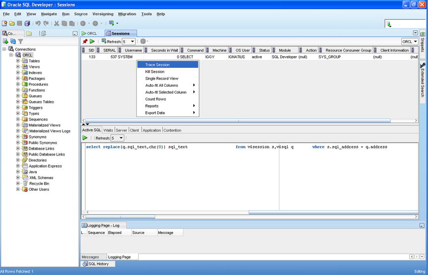
Figure 17-1. Using SQL Developer to monitor sessions
A systematic way of identifying tuning candidates in a batch job is to trace the job. If you ask Oracle to trace a job, it records SQL statements and execution details in a trace file. The simplest way to start tracing a session is to use Enterprise Manager or SQL Developer as in Figure 17-1. You can also use the SET_SQL_TRACE_IN_SESSION command as in the following example:
EXECUTE dbms_system.set_sql_trace:in_session(133, 537, true);
You can then use the tkprof tool to summarize the information in a more readable form, as in Listing 17-1. You can see that a particular statement was executed 163 times—execution statistics are also displayed. In this case, the number of logical reads—the number of buffers gotten for consistent read—is zero because the information is coming from dynamic performance tables, not from actual database tables.
Another way to identify tuning candidates is to examine a Statspack or Automatic Workload Repository (AWR) report. They were discussed in Chapter 16.
Understanding the Causes of Inefficient SQL
You may not even realize that you are dealing with inefficient SQL because powerful hardware can compensate for much inefficiency. In fact, one simple method of “improving” performance is simply to throw powerful hardware at the problem.1 In other cases, a statement may take so little time to execute that you may not realize it is inefficient. There are many different causes for poor performance of SQL statements, and there are many solutions; a short discussion cannot do them justice.
Also keep in mind that, given enough time, effort, and money, it is always possible to extract more performance from an SQL statement. The example used in this chapter perfectly illustrates the point; you keep improving its performance until you hit the theoretical maximum level of performance. However, it is not usually possible to give so much time and attention to individual statements. The amount of effort you are willing to expend is usually governed by business requirements and the return on your investment.
The most frequently cited cause of inefficient SQL is the failure of the query optimizer to generate an efficient query-execution plan, but there are many others. Here are some examples:
- There are usually many ways to write the same query, and not all of them are equally efficient. Failure to use advanced features of the language is a common cause of inefficient SQL.
- Poor application-development practices may increase the amount of inefficient SQL. For example, giving users the ability to generate new types of queries (a.k.a. ad hoc queries) is usually a perfect recipe for poor performance. Another example of poor application-development practices is insufficient testing.
- Logical and physical database design can play a big role in SQL performance. Examples are inadequate indexing and partitioning of data, and insufficient attention to disk layouts.
- Inadequate database maintenance can cause SQL performance to degrade as time passes. A perfect example is the absence of an archiving strategy to keep the amount of data under control.
It bears repeating that hardware limitations—including CPU speed, memory size, and disk speed—play a big role in performance. If the system does not have enough memory, data may have to be frequently retrieved from disk. The workload handled by the database server also plays a major role in performance; your SQL statement will run slowly if it has to compete for resources with SQL statements submitted by other users. Often this is the result of poor coordination of workloads. For example, it is poor practice to perform batch processing during the day when most OLTP work is performed. Sometimes this is the result of poor capacity planning. For example, an online store may not have properly planned for the increase in transaction volumes during popular holidays.
Ways to Improve SQL
Given enough time, effort, and money, it is usually possible to extract more performance from any SQL statement. However, it is not usually possible to give so much time and attention to individual statements. The amount of effort you are willing to expend is usually governed by business requirements and the return on your investment. The goal is usually to bring performance of poorly performing SQL statements to a level that is acceptable to the users of the database. The following sections describe some techniques that can be used to improve performance.
Indexes
A common reason for inefficient processing of SQL statements is the lack of appropriate indexes and other paths to reach the required data. Imagine how difficult it would be to find an item of information in a book if those items were not organized into appropriate chapters and there was no index of key words at the back of the book. Chapter 7 discussed indexes.
Most tables have a primary key and therefore have at least one index—that is, the index on the items composing the primary key. This index is used to ensure that no two records contain the same values of these data items. The absence of such an index would make it harder to ensure this. Indexes should also be created for any foreign keys in a table—that is, data items that link the table to another table—unless the table in question is small enough that the lack of such indexes will not have an impact on performance. Indexes should also be created for data items that are restricted in SQL queries.
The dba_indexes and dba_ind_columns views show what indexes have been created, as in the following example from the tuning exercise in this chapter:
SQL> SELECT table_name,
  2         index_name
  3    FROM user_indexes
  4   WHERE table_name in (’MY_TABLES’, ’MY_INDEXES’);

TABLE_NAME           INDEX_NAME
-------------------- --------------------
MY_INDEXES           MY_INDEXES_FK1
MY_INDEXES           MY_INDEXES_I1
MY_INDEXES           MY_INDEXES_PK
MY_TABLES            MY_TABLES_PK

SQL> SELECT table_name,
  2         index_name,
  3         column_name,
  4         column_position
  5    FROM user_ind_columns
  6   WHERE table_name in (’MY_TABLES’, ’MY_INDEXES’);

TABLE_NAME           INDEX_NAME           COLUMN_NAME          COLUMN_POSITION
-------------------- -------------------- -------------------- ---------------
MY_INDEXES           MY_INDEXES_PK        OWNER                              1
MY_INDEXES           MY_INDEXES_PK        INDEX_NAME                         2
MY_INDEXES           MY_INDEXES_I1        INDEX_TYPE                         1
MY_INDEXES           MY_INDEXES_FK1       TABLE_OWNER                        1
MY_INDEXES           MY_INDEXES_FK1       TABLE_NAME                         2
MY_TABLES            MY_TABLES_PK         OWNER                              1
MY_TABLES            MY_TABLES_PK         TABLE_NAME                         2
Database designers have several kinds of indexes at their disposal. The most common are listed here:
- Most indexes are of the b*tree (balanced tree) type and are best suited for online transaction-processing environments. Index entries are stored in a structure that has a root node, branches, and leaves; hence the name.
- Reverse key indexes are a specialized type of b*tree index in which the key values are reversed (for example, IGGY becomes YGGI) to prevent concentrations of similar entries in index blocks and consequent contention for blocks.
- Function-based indexes and indexes on virtual columns (columns defined in terms of other columns) are indexes not on the data values contained in columns but on combinations of these values. For example, an index on UPPER(name) is an example of a function-based index.
- Bitmap indexes are a specialized kind of index used in data warehouses for columns that contain only a few values—for example, model, year, and color. Each value is represented by a bitmap (an array of 0s and 1s), and each element of the bitmap represents one record in the table.
In addition to indexes, database designers have other data structures at their disposal. Examples include clusters, index-organized tables, and partitioned tables.
![]() Tip Oracle does not use an index unless the query optimizer perceives a benefit in doing so. You can verify that an index is being used by issuing the MONITORING USAGE clause of the ALTER INDEX command and reviewing the contents of the v$object_usage view after a suitable time has passed. If Oracle is not using an index, you can use the techniques in the following sections to increase the chances that it will do so. If an index is never used, you should consider whether it can be removed safely, because indexes slow down insert, update, and delete operations and occupy valuable space within the database.
Tip Oracle does not use an index unless the query optimizer perceives a benefit in doing so. You can verify that an index is being used by issuing the MONITORING USAGE clause of the ALTER INDEX command and reviewing the contents of the v$object_usage view after a suitable time has passed. If Oracle is not using an index, you can use the techniques in the following sections to increase the chances that it will do so. If an index is never used, you should consider whether it can be removed safely, because indexes slow down insert, update, and delete operations and occupy valuable space within the database.
Hints
Hints for the optimizer can be embedded inside an SQL statement if the optimizer does not find an acceptable query plan for the statement. Each hint partially constrains the optimizer, and a full set of hints completely constrains the optimizer. In fact, a desirable query plan can be preserved by capturing the complete set of hints that describes it in a stored outline. For details, refer to Oracle Database 12c Performance Tuning Guide.
The most commonly used hints are in the following list. You can find detailed information on these and other hints in Oracle Database 12c SQL Language Reference:
- The LEADING hint instructs Oracle to process the specified tables first, in the order listed.
- The ORDERED hint instructs Oracle to process the tables in the order listed in the body of the SQL statement.
- The INDEX hint instructs Oracle to use the specified index when processing the specified table.
- The FULL hint instructs Oracle not to use indexes when processing the specified table.
- The NO_MERGE hint instructs Oracle to optimize and process an inline view separately from the rest of the query.
- The USE_NL, USE_HASH, and USE_MERGE hints are used in conjunction with the LEADING hint or the ORDERED hint to constrain the choice of join method (nested loops, hash, or sort-merge) for the specified table.
Here is an example of an SQL query that incorporates hints to guide and constrain the optimizer. Oracle is instructed to visit the my_indexes table before the my_tables table. Oracle is also instructed to use an index on the index_type data item in my_indexes and an index on the owner and table_name data items in my_tables, if such indexes are available. Note that hints must come directly after the SELECT keyword and must be enclosed between special markers—for example, /*+ INDEX(MY_INDEXES (INDEX_TYPE)) */:
SELECT          /*+ INDEX(MY_INDEXES (INDEX_TYPE))
                    INDEX(MY_TABLES (OWNER TABLE_NAME))
                    LEADING(MY_INDEXES MY_TABLES)
                    USE_NL(MY_TABLES)
                */
       DISTINCT my_tables.owner,
                my_tables.table_name,
                my_tables.tablespace:name
           FROM my_tables, my_indexes
          WHERE my_tables.owner = my_indexes.table_owner
            AND my_tables.table_name = my_indexes.table_name
            AND my_indexes.index_type = :index_type;
Statistics
Statistical information on tables and indexes and the data they contain is what the query optimizer needs to do its job properly. The simplest way to collect statistics is to use the procedures in the DBMS_STATS package. For example, DBMS_STATS.GATHER_TABLE_STATS can be used to collect statistics for a single table, and DBMS_STATS.GATHER_SCHEMA_STATS can be used to collect statistics for all the tables in a schema. You see some examples in the tuning exercise in this chapter.
However, the question of how and when to collect statistics does not have an easy answer, because changes in statistics can lead to changes in query-execution plans that are not always for the better. A perfect example of how fresh statistics can degrade performance occurs when statistics are collected on a table that contains very volatile data. The statistics describe the data that existed when the statistics were collected, but the data could change soon thereafter; the table could be empty when the statistics were collected but could be filled with data soon thereafter.
Here is what various Oracle experts have said on the subject. The quote that ties all the other quotes together is the last. You have to understand your data in order to create a strategy that works best for your situation:
It astonishes me how many shops prohibit any unapproved production changes and yet reanalyze schema stats weekly. Evidently, they do not understand that the purpose of schema reanalysis is to change their production SQL execution plans, and they act surprised when performance changes!2
I have advised many customers to stop analyzing, thereby creating a more stable environment overnight.3
Oh, and by the way, could you please stop gathering statistics constantly? I don’t know much about databases, but I do think I know the following: small tables tend to stay small, large tables tend to stay large, unique indexes have a tendency to stay unique, and nonunique indexes often stay nonunique.4
Monitor the changes in execution plans and/or performance for the individual SQL statements…and perhaps as a consequence regather stats. That way, you’d leave stuff alone that works very well, thank you, and you’d put your efforts into exactly the things that have become worse.5
It is my firm belief that most scheduled statistics-gathering jobs do not cause much harm only because (most) changes in the statistics were insignificant as far as the optimizer is concerned—meaning that it was an exercise in futility.6
There are some statistics about your data that can be left unchanged for a long time, possibly forever; there are some statistics that need to be changed periodically; and there are some statistics that need to be changed constantly…. The biggest problem is that you need to understand the data.7
Beginning with Oracle 10g, statistics are automatically collected by a job that runs during a nightly maintenance window. This default strategy may work for many databases. You can use the procedures in the DBMS_STATS package to create a custom strategy. Complete details of the DBMS_STATS package can be found in Oracle Database PL/SQL Packages and Types Reference. Here is a representative list of the available procedures:
- The GATHER_*_STATS procedures can be used to manually gather statistics. For example, GATHER_TABLE_STATS gathers statistics for a single table, and GATHER_SCHEMA_STATS gathers statistics for all the indexes and tables in a schema.
- The DELETE_*_STATS procedures can be used to delete statistics.
- The EXPORT_*_STATS procedures can be used to copy the statistics to a special table. IMPORT_*_STATS can be used to import desired statistics. For example, statistics can be exported from a production database and imported into a development database; this ensures that both databases use the same query-execution plans.
- The GATHER_STATS_JOB job retains previous statistics. The RESTORE_*_STATS procedures can be used to restore statistics from a previous point in time. The default retention period used by the GATHER_STATS_JOB is 31 days; you can change this by using the ALTER_STATS_HISTORY_RETENTION procedure.
- The LOCK_*_STATS procedures can be used to lock statistics and prevent them from being overwritten. Oddly enough, locking statistics can be a useful practice not only when data is static, but also when it is volatile.
- Possibly the most important procedures are the SET_*_PREFS procedures. They can be used to customize how the GATHER_STATS_JOB collects statistics. The available options are similar to those of the GATHER_*_STATS procedures.
![]() Caution One class of statistics that is not collected automatically is the system statistics. An example is sreadtim, the time taken to read one random block from disk. You can must collect system statistics manually by using the GATHER_SYSTEM_STATS procedure. For details, refer to Oracle Database 12c PL/SQL Packages and Types Reference.
Caution One class of statistics that is not collected automatically is the system statistics. An example is sreadtim, the time taken to read one random block from disk. You can must collect system statistics manually by using the GATHER_SYSTEM_STATS procedure. For details, refer to Oracle Database 12c PL/SQL Packages and Types Reference.
Tuning by Example
Let’s experience the process of tuning an SQL statement by creating two tables, my_tables and my_indexes, modeled after dba_tables and dba_indexes, two dictionary views. Every record in my_tables describes one table, and every record in my_indexes describes one index. The exercise is to print the details (owner, table_name, and tablespace:name) of tables that have at least one bitmap index.
Note that the SELECT ANY DICTIONARY, ALTER SYSTEM , ADVISOR, and CREATE CLUSTER privileges are needed for this exercise. Connect as SYSTEM, and grant them to the HR account. Also take a minute to extend the password expiry date of the HR account; if you neglect to do so, you will receive the message “ORA-28002: the password will expire within 7 days” when you connect to the HR account and will not be able to use the autotrace feature required for this exercise:
[oracle@localhost ~]$ sqlplus system/oracle@pdb1

SQL*Plus: Release 12.1.0.1.0 Production on Sun Feb 1 12:20:00 2015

Copyright (c) 1982, 2013, Oracle.  All rights reserved.

Last Successful login time: Sun Feb 01 2015 12:19:50 -05:00

Connected to:
Oracle Database 12c Enterprise Edition Release 12.1.0.1.0 - 64bit Production
With the Partitioning, OLAP, Advanced Analytics and Real Application Testing options

PDB1@ORCL> grant select any dictionary to hr;

Grant succeeded.

PDB1@ORCL> grant alter system to hr;

Grant succeeded.

PDB1@ORCL> alter user hr identified by oracle;

User altered.

PDB1@ORCL> grant advisor to hr;

Grant succeeded.

PDB1@ORCL> grant create cluster to hr;

Grant succeeded.

PDB1@ORCL> exit
Disconnected from Oracle Database 12c Enterprise Edition Release 12.1.0.1.0 - 64bit Production
With the Partitioning, OLAP, Advanced Analytics and Real Application Testing options
You also need to create a role called plustrace in order to trace SQL statements in SQL*Plus. Log in to the SYS account, and execute the plustrace.sql script in the sqlplus/admin folder in ORACLE_HOME. Then grant the newly created plustrace role to public:
[oracle@localhost ~]$ sqlplus sys/oracle@pdb1 as sysdba

SQL*Plus: Release 12.1.0.1.0 Production on Sun Feb 1 13:43:46 2015

Copyright (c) 1982, 2013, Oracle.  All rights reserved.

Connected to:
Oracle Database 12c Enterprise Edition Release 12.1.0.1.0 - 64bit Production
With the Partitioning, OLAP, Advanced Analytics and Real Application Testing options

PDB1@ORCL> @?/sqlplus/admin/plustrce
PDB1@ORCL>
PDB1@ORCL> drop role plustrace;
drop role plustrace
          *
ERROR at line 1:
ORA-01919: role ’PLUSTRACE’ does not exist

PDB1@ORCL> create role plustrace;

Role created.

PDB1@ORCL>
PDB1@ORCL> grant select on v_$sesstat to plustrace;

Grant succeeded.

PDB1@ORCL> grant select on v_$statname to plustrace;

Grant succeeded.

PDB1@ORCL> grant select on v_$mystat to plustrace;

Grant succeeded.

PDB1@ORCL> grant plustrace to dba with admin option;

Grant succeeded.

PDB1@ORCL>
PDB1@ORCL> set echo off
PDB1@ORCL> grant plustrace to public;

Grant succeeded.

PDB1@ORCL> exit
Disconnected from Oracle Database 12c Enterprise Edition Release 12.1.0.1.0 - 64bit Production
With the Partitioning, OLAP, Advanced Analytics and Real Application Testing options
Creating and Populating the Tables
Create and populate the two tables as follows. When I performed the experiment, 2,371 records were inserted into my_tables, and 3,938 records were inserted into my_indexes:
PDB1@ORCL> CREATE TABLE my_tables AS
  2  SELECT dba_tables.* FROM dba_tables;

Table created.

PDB1@ORCL> CREATE TABLE my_indexes AS
  2  SELECT dba_indexes.*
  3  FROM dba_tables,
  4    dba_indexes
  5  WHERE dba_tables.owner    = dba_indexes.table_owner
  6  AND dba_tables.table_name = dba_indexes.table_name;

Table created.

PDB1@ORCL> /* Count the records in the my_tables table */
PDB1@ORCL> SELECT COUNT(*) FROM my_tables;

  COUNT(*)
----------
      2371

PDB1@ORCL> /* Count the records in the my_indexes table */
PDB1@ORCL> SELECT COUNT(*) FROM my_indexes;

  COUNT(*)
----------
      3938
Establishing a Baseline
Here is a simple SQL statement that prints the required information (owner, table_name, and tablespace:name) about tables that have an index of a specified type. You join my_tables and my_indexes, extract the required pieces of information from my_tables, and eliminate duplicates by using the DISTINCT operator:
SELECT DISTINCT my_tables.owner,
  my_tables.table_name,
  my_tables.tablespace:name
FROM my_tables,
  my_indexes
WHERE my_tables.owner     = my_indexes.table_owner
AND my_tables.table_name  = my_indexes.table_name
AND my_indexes.index_type = :index_type
Observe that you have not yet created appropriate indexes for my_tables and my_indexes, nor have you collected statistical information for use in constructing query-execution plans. However, you will soon see that Oracle can execute queries and join tables even in the absence of indexes and can even generate statistical information dynamically by sampling the data.
Some preliminaries are required before you execute the query. You must activate the autotrace feature and must ensure that detailed timing information is captured during the course of the query (statistics_level=ALL). The autotrace feature is used to print the most important items of information relating to efficiency of SQL queries. More-detailed information is captured by Oracle if statistics_level is appropriately configured:
PDB1@ORCL> ALTER SESSION SET statistics_level=ALL;

Session altered.

PDB1@ORCL> SET AUTOTRACE ON statistics
PDB1@ORCL> VARIABLE index_type VARCHAR2(32);
PDB1@ORCL> EXEC :index_type := ’FUNCTION-BASED NORMAL’;

PL/SQL procedure successfully completed.

PDB1@ORCL> column owner format a30
PDB1@ORCL> column table_name format a30
PDB1@ORCL> column tablespace:name format a30
PDB1@ORCL> set linesize 100
PDB1@ORCL> set pagesize 100
PDB1@ORCL> SELECT DISTINCT my_tables.owner,
  2    my_tables.table_name,
  3    my_tables.tablespace:name
  4  FROM my_tables,
  5    my_indexes
  6  WHERE my_tables.owner     = my_indexes.table_owner
  7  AND my_tables.table_name  = my_indexes.table_name
  8  AND my_indexes.index_type = :index_type;
s
OWNER                          TABLE_NAME                     TABLESPACE_NAME
------------------------------ ------------------------------ ------------------------------
SYS                            WRI$_OPTSTAT_TAB_HISTORY       SYSAUX
SYS                            XS$NSTMPL_ATTR                 SYSTEM
XDB                            X$PT6UFI5W7S9D1VDE0GP5LBK0KHIF SYSAUX
WMSYS                          WM$CONSTRAINTS_TABLE$          SYSAUX
SYS                            SCHEDULER$_JOB                 SYSTEM
WMSYS                          WM$HINT_TABLE$                 SYSAUX
APEX_040200                    WWV_FLOW_LIST_OF_VALUES_DATA   SYSAUX
SYS                            WRI$_OPTSTAT_HISTGRM_HISTORY
SYS                            WRI$_OPTSTAT_OPR               SYSAUX
SYS                            WRI$_OPTSTAT_OPR_TASKS         SYSAUX
SYS                            SCHEDULER$_WINDOW              SYSTEM
WMSYS                          WM$VERSIONED_TABLES$           SYSAUX
APEX_040200                    WWV_FLOW_WORKSHEET_RPTS        SYSAUX
APEX_040200                    WWV_FLOW_COMPANY_SCHEMAS       SYSAUX
OBE                            OEHR_CUSTOMERS                 APEX_2264528630961551
APEX_040200                    WWV_FLOW_MAIL_LOG              SYSAUX
SYS                            XS$ACL_PARAM                   SYSTEM
SYS                            WRI$_OPTSTAT_HISTHEAD_HISTORY
SYS                            WRI$_OPTSTAT_IND_HISTORY       SYSAUX
SYS                            WRI$_OPTSTAT_AUX_HISTORY       SYSAUX
SYS                            DBFS$_MOUNTS                   SYSTEM
APEX_040200                    WWV_FLOW_REPORT_LAYOUTS        SYSAUX
APEX_040200                    WWV_FLOW_WORKSHEETS            SYSAUX
APEX_040200                    WWV_FLOW_WORKSHEET_CONDITIONS  SYSAUX

24 rows selected.

Statistics
----------------------------------------------------------
          4  recursive calls
        238  consistent gets
          0  physical reads
          0  db block gets
        124  redo size
       1768  bytes sent via SQL*Net to client
        554  bytes received via SQL*Net from client
          3  SQL*Net roundtrips to/from client
          0  sorts (memory)
          0  sorts (disk)
         24  rows processed
Twenty-four rows of data are printed. The name of the tablespace is not printed in the case of two tables; the explanation is left as an exercise for you. But the more interesting information is that relating to the efficiency of the query. This is printed because you activated the autotrace feature. Here is an explanation of the various items of information:
- Recursive calls are all the internal queries that are executed behind the scenes in addition to your query. When a query is submitted for execution, Oracle first checks its syntax. It then checks the semantics—that is, it de-references synonyms and views and identifies the underlying tables. It then computes the signature (a.k.a. hash value) of the query and checks its cache of query-execution plans for a reusable query plan that corresponds to that signature. If a query plan is not found, Oracle has to construct one; this results in recursive calls. The number of recursive calls required can be large if the information Oracle needs to construct the query plan is not available in the dictionary cache and has to be retrieved from the database or if there are no statistics about tables mentioned in the query and data blocks have to be sampled to generate statistics dynamically.
- DB block gets is the number of times Oracle needs the latest version of a data block. Oracle does not need the latest version of a data block when the data is simply being read by the user. Instead, Oracle needs the version of the data block that was current when the query started. The latest version of a data block is typically required when the intention is to modify the data. Note that db block gets is 0 in all the examples in this chapter.
- Consistent gets, a.k.a. logical reads, is the number of operations to retrieve a consistent version of a data block that were performed by Oracle while constructing query plans and while executing queries. Remember that all data blocks read during the execution of any query are the versions that were current when the query started; this is called read consistency. One of the principal objectives of query tuning is to reduce the number of consistent get operations that are required.
- Physical reads is the number of operations to read data blocks from the disks that were performed by Oracle because the blocks were not found in Oracle’s cache when they were required. The limit on the number of physical reads is therefore the number of consistent gets.
- Redo size is the amount of information Oracle writes to the journals that track changes to the database. This metric applies only when the data is changed in some way.
- Bytes sent via SQL*Net to client, bytes received via SQL*Net from client, and SQL*Net roundtrips to/from client are fairly self-explanatory; they track the number and size of messages sent to and from Oracle and the user.
- Sorts (memory) and sorts (disk) track the number of sorting operations performed by Oracle during the course of your query. Sorting operations are performed in memory if possible; they spill onto the disks if the data does not fit into Oracle’s memory buffers. It is desirable for sorting to be performed in memory because reading and writing data to and from the disks are expensive operations. The amount of memory available to database sessions for sorting operations is controlled by the value of PGA_AGGREGATE_TARGET.
- Rows processed is the number of rows of information required by the user.
The preceding explanations should make it clear that a lot of overhead is involved in executing a query—for example, physical reads are required if data blocks are not found in Oracle’s cache. The amount of overhead during any execution varies depending on the contents of the shared pool (cache of query-execution plans) and buffer cache (cache of data blocks) at the time of execution. You can gauge the complete extent of overhead by flushing both the shared pool and buffer cache and then re-executing the query:
PDB1@ORCL> ALTER SYSTEM FLUSH SHARED_POOL;

System altered.

PDB1@ORCL> ALTER SYSTEM FLUSH BUFFER_CACHE;

System altered.
After the flush, 201 recursive calls, 344 consistent gets (including 237 physical reads), and 10 sort operations are required:
Statistics
----------------------------------------------------------
        190  recursive calls
          0  db block gets
        344  consistent gets
        237  physical reads
          0  redo size
       1768  bytes sent via SQL*Net to client
        554  bytes received via SQL*Net from client
          3  SQL*Net roundtrips to/from client
         10  sorts (memory)
          0  sorts (disk)
         24  rows processed
Let’s now flush only the buffer cache and execute the query again to quantify the precise amount of overhead work involved in constructing a query-execution plan. Recursive calls and sorts fall from 1,653 to 0, and consistent gets fall from 498 to 108. The amount of overhead work dwarfs the actual work done by the query. The number of consistent gets is 108; it will not decrease if you repeat the query again. The baseline number that you will attempt to reduce in this tuning exercise is therefore 108. Notice that the number of physical reads is less than the number of consistent gets even though you flushed the buffer cache before executing the query. The reason is that the consistent gets metric counts a block as many times as it is accessed during the course of a query, whereas the physical reads metric counts a block only when it is brought into the buffer cache from the disks. A block might be accessed several times during the course of the query but might have to be brought into the buffer cache only once:
Statistics
----------------------------------------------------------
          1  recursive calls
          0  db block gets
        228  consistent gets
        222  physical reads
          0  redo size
       1768  bytes sent via SQL*Net to client
        554  bytes received via SQL*Net from client
          3  SQL*Net roundtrips to/from client
          0  sorts (memory)
          0  sorts (disk)
         24  rows processed
Executing the query yet one more time, we see that physical reads has fallen to zero because all data blocks are found in Oracle’s cache:
Statistics
----------------------------------------------------------
          0  recursive calls
          0  db block gets
        228  consistent gets
          0  physical reads
          0  redo size
       1768  bytes sent via SQL*Net to client
        554  bytes received via SQL*Net from client
          3  SQL*Net roundtrips to/from client
          0  sorts (memory)
          0  sorts (disk)
         24  rows processed
Table 17-1 summarizes the findings. The first time you executed the query, Oracle had to construct a query-execution plan but found most of the required dictionary information in its cache. The second time you executed the query, Oracle had to reread all the dictionary execution into cache—this explains the recursive calls and the physical reads—as well as all the data blocks required during the actual execution of the query. The third time you executed the query, Oracle did not have to construct an execution plan, but all the data bocks required during the execution of the query had to be obtained from disk. The fourth time you executed the query, all the required data blocks were found in Oracle’s cache.
Table 17-1. Overhead Work Required to Construct a Query-Execution Plan
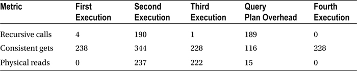
The number of consistent gets will not go down if you repeat the query a fifth time; 228 is therefore the baseline number you will try to reduce in this tuning exercise.
Examining the Query Plan
It is now time to examine the query plan that Oracle has been using. A simple way to do so is to use the dbms_xplan.display_cursor procedure. The following query plan was displayed after I flushed the shared pool and the buffer cache earlier in the exercise.
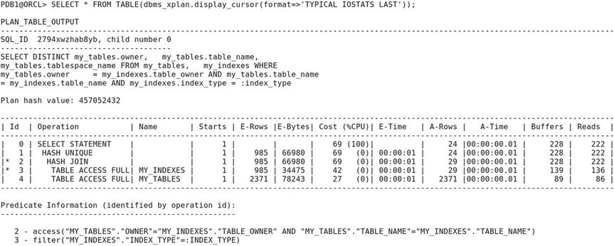
The hash signature (SQL_ID) of the SQL statement is 2794xwzhab8yb, and that of the query execution plan is 457052432. You may obtain different values when you try the exercise in your database. Oracle caches as many plans as possible for future reuse and knows how to translate a hash value into the precise place in memory where the SQL statement or plan is stored. Whenever an SQL statement is submitted for execution, Oracle computes its signature and searches for a statement with identical text and semantics in the cache. If a statement with identical text and semantics is found, its plan can be reused. If Oracle finds a statement with identical text but does not find one that also has identical semantics, it must create a new execution plan; this execution plan is called a child cursor. Multiple plans can exist for the same statement—this is indicated by the child number. For example, two users may each own a private copy of a table mentioned in an SQL statement, and therefore different query plans are needed for each user.
The execution plan itself is shown in tabular format and is followed by the list of filters (a.k.a. predicates) that apply to the rows of the table. Each row in the table represents one step of the query-execution plan. Here is the description of the columns:
- Id is the row number.
- Operation describes the step—for example, TABLE ACCESS FULL means all rows in the table are retrieved.
- Name is an optional piece of information; it is the name of the object to which the step applies.
- Starts is the number of times the step is executed.
- E-Rows is the number of rows that Oracle expected to obtain in the step.
- E-Bytes is the total number of bytes that Oracle expected to obtain in the step.
- Cost is the cumulative cost that Oracle expected to incur at the end of the step. The unit is best understood as the estimated time to read a single block from disk (sreadtim) recorded in the “system statistics.” In other words, the cost is the number of data blocks that could be retrieved in the time that Oracle expects . The percentage of time for which Oracle expects to use the CPU is displayed along with the cost.
- E-Time is an estimate of the cumulative amount of time to complete this step and all prior steps. Hours, minutes, and seconds are displayed.
- A-Rows is the number of rows that Oracle actually obtained in the step.
- A-Bytes is the total number of bytes that Oracle actually obtained in the step.
- Buffers is the cumulative number of consistent get operations that were actually performed in the step and all prior steps.
- Reads is the cumulative number of physical read operations that were actually performed in the step and all prior steps.
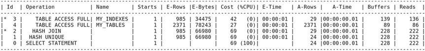
A little skill is needed to interpret the execution plan. Notice the indentation of the operations listed in the second column. The correct sequence of operations is obtained by applying the following rule: perform operations in the order in which they are listed, except that if the operations listed after a certain operation are more deeply indented in the listing, then perform those operations first (in the order in which those operations are listed). On applying this rule, you see that the operations are performed in the following order:
First, all the rows of data in the my_indexes table are retrieved (TABLE ACCESS FULL), and a lookup table (a.k.a. hash table) is constructed from rows that satisfy the filter (a.k.a. predicate) my_indexes.index_type = :index_type. This means a signature (a.k.a. hash value) is calculated for each row of data satisfying the predicate. This signature is then translated into a position in the hash table where the row will be stored. This makes it tremendously easy to locate the row when it is required later. Because my_indexes and my_tables are related by the values of owner and table_name, a hash signature is constructed from these values.
Next, all the rows of data in the my_tables table are retrieved (TABLE ACCESS FULL). After retrieving each row of data from the my_tables table, rows of data from the my_indexes table satisfying the join predicate my_tables.owner = my_indexes.owner AND my_tables.table_name = my_indexes.table_name are retrieved from the lookup table constructed in the previous step (HASH JOIN); and if any such rows are found, the required data items (owner, table_name, and tablespace:name) are included in the query results. Duplicates are avoided (HASH UNIQUE) by storing the resulting rows of data in another hash table; new rows are added to the hash table only if a matching row is not found.
Of particular interest are the columns in the execution plan labeled E-Rows, E-Bytes, Cost, and E-Time. These are estimates generated by Oracle. Time and cost are straightforward computations based on rows and bytes, but how does Oracle estimate rows and bytes in the first place? The answer is that Oracle uses a combination of rules of thumb and any available statistical information available in the data dictionary; this statistical information is automatically refreshed every night by default. In the absence of statistical information, Oracle samples a certain number of data blocks from the table and estimates the number of qualifying rows in each block of the table and the average length of these rows; this is referred to as dynamic sampling.
Observe the values in the E-Rows and A-Rows columns in the execution plan. Oracle’s estimate of the number of qualifying rows in my_tables is surprisingly accurate. The reason is that Oracle Database 12c automatically generates statistics during a CREATE TABLE AS SELECT (CTAS) operation. However, there are wide discrepancies between the E-Rows and A-Rows values in other lines of the execution plan.
Indexes and Statistics
Let’s create an appropriate set of indexes on your tables. First you define primary key constraints on my_tables and my_indexes. Oracle automatically creates unique indexes because it needs an efficient method of enforcing the constraints. You also create a foreign-key constraint linking the two tables and create an index on the foreign key. Finally, you create an index on the values of index_type because your query restricts the value of index_type. You then refresh statistics on both tables:
ALTER TABLE my_tables
ADD (CONSTRAINT my_tables_pk PRIMARY KEY (owner, table_name));

ALTER TABLE my_indexes
ADD (CONSTRAINT my_indexes_pk PRIMARY KEY (owner, index_name));

ALTER TABLE my_indexes
ADD (CONSTRAINT my_indexes_fk1 FOREIGN KEY (table_owner, table_name)
REFERENCES my_tables);

CREATE INDEX my_indexes_i1 ON my_indexes (index_type);

CREATE INDEX my_indexes_fk1 ON my_indexes (table_owner, table_name);

EXEC DBMS_STATS.gather_table_stats(user,tabname=>’MY_TABLES’);
EXEC DBMS_STATS.gather_table_stats(user,tabname=>’MY_INDEXES’);
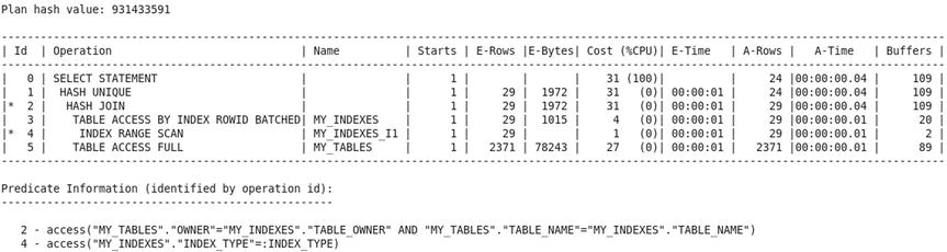
You find tremendous improvement in the accuracy of the estimates and a substantial improvement in the efficiency of the query plan after indexes are created and statistics are gathered. Oracle now correctly estimates that 29 rows will be retrieved from the my_indexes table. Oracle uses the index on the values of index_type to efficiently retrieve the 15 qualifying rows. This execution plan requires only 109 consistent gets.
Using SQL Access Advisor
If you are using Enterprise Edition and have a license for the Tuning Pack, you can use a feature called SQL Tuning Advisor to help you with SQL tuning. You’ve already created indexes and generated statistics; you can now look to SQL Tuning Advisor for fresh ideas. SQL Advisor finds a better plan that reduces the number of consistent gets to 80 and creates a profile that, if accepted, will increase the likelihood that the better plan is chosen. This profile consists of OPT_ESTIMATE hints, which are scaling factors that are used to adjust the calculations of the optimizer. The next section shows how explicit hints can be used to obtain this plan:
PDB1@ORCL> VARIABLE tuning_task VARCHAR2(32);
PDB1@ORCL> EXEC :tuning_task := dbms_sqltune.create_tuning_task (sql_id => ’2794xwzhab8yb’);

PL/SQL procedure successfully completed.

PDB1@ORCL> EXEC dbms_sqltune.execute_tuning_task(task_name => :tuning_task);

PL/SQL procedure successfully completed.

PDB1@ORCL> SET LONG 100000;
PDB1@ORCL> SET PAGESIZE 1000
PDB1@ORCL> SET LINESIZE 200
PDB1@ORCL> COLUMN recommendations FORMAT a200
PDB1@ORCL> SELECT DBMS_SQLTUNE.report_tuning_task (:tuning_task) AS recommendations FROM DUAL;

RECOMMENDATIONS
-------------------------------------------------------------------------------
GENERAL INFORMATION SECTION
-------------------------------------------------------------------------------
Tuning Task Name   : TASK_11
Tuning Task Owner  : HR
Workload Type      : Single SQL Statement
Scope              : COMPREHENSIVE
Time Limit(seconds): 1800
Completion Status  : COMPLETED
Started at         : 04/12/2015 21:33:14
Completed at       : 04/12/2015 21:33:21

-------------------------------------------------------------------------------
Schema Name   : HR
Container Name: PDB1
SQL ID        : 2794xwzhab8yb
SQL Text      : SELECT DISTINCT my_tables.owner,
                  my_tables.table_name,
                  my_tables.tablespace:name
                FROM my_tables,
                  my_indexes
                WHERE my_tables.owner     = my_indexes.table_owner
                AND my_tables.table_name  = my_indexes.table_name
                AND my_indexes.index_type = :index_type
Bind Variables: :
 1 -  (VARCHAR2(128)):FUNCTION-BASED NORMAL

-------------------------------------------------------------------------------
FINDINGS SECTION (1 finding)
-------------------------------------------------------------------------------

1- SQL Profile Finding (see explain plans section below)
--------------------------------------------------------
  A potentially better execution plan was found for this statement.

  Recommendation (estimated benefit: 28.5%)
  -----------------------------------------
  - Consider accepting the recommended SQL profile.
    execute dbms_sqltune.accept_sql_profile(task_name => ’TASK_11’,
            task_owner => ’HR’, replace => TRUE);

  Validation results
  ------------------
  The SQL profile was tested by executing both its plan and the original plan
  and measuring their respective execution statistics. A plan may have been
  only partially executed if the other could be run to completion in less time.

                           Original Plan  With SQL Profile  % Improved
                           -------------  ----------------  ----------
  Completion Status:            COMPLETE          COMPLETE
  Elapsed Time (s):             .033816           .002418      92.84 %
  CPU Time (s):                   .0319             .0021      93.41 %
  User I/O Time (s):                  0                 0
  Buffer Gets:                      109                80       26.6 %
  Physical Read Requests:             0                 0
  Physical Write Requests:            0                 0
  Physical Read Bytes:                0                 0
  Physical Write Bytes:               0                 0
  Rows Processed:                    24                24
  Fetches:                           24                24
  Executions:                         1                 1

  Notes
  -----
  1. Statistics for the original plan were averaged over 10 executions.
  2. Statistics for the SQL profile plan were averaged over 10 executions.

-------------------------------------------------------------------------------
EXPLAIN PLANS SECTION
-------------------------------------------------------------------------------

2- Using SQL Profile
--------------------
Plan hash value: 3284819692

-------------------------------------------------------------------------------
| Id  | Operation                     | Name          | Rows  | Bytes | Cost  |
-------------------------------------------------------------------------------
|   0 | SELECT STATEMENT              |               |    29 |  1972 |    37 |
|   1 |  SORT UNIQUE                  |               |    29 |  1972 |    37 |
|   2 |   NESTED LOOPS                |               |    29 |  1972 |    33 |
|   3 |    TABLE ACCESS BY INDEX ROWID| MY_INDEXES    |    29 |  1015 |     4 |
|*  4 |     INDEX RANGE SCAN          | MY_INDEXES_I1 |    29 |       |     1 |
|   5 |    TABLE ACCESS BY INDEX ROWID| MY_TABLES     |     1 |    33 |     1 |
|*  6 |     INDEX UNIQUE SCAN         | MY_TABLES_PK  |     1 |       |       |
-------------------------------------------------------------------------------

Predicate Information (identified by operation id):
---------------------------------------------------

   4 - access("MY_INDEXES"."INDEX_TYPE"=:INDEX_TYPE)
   6 - access("MY_TABLES"."OWNER"="MY_INDEXES"."TABLE_OWNER" AND
              "MY_TABLES"."TABLE_NAME"="MY_INDEXES"."TABLE_NAME")

-------------------------------------------------------------------------------
Optimizer Hints
Hints for the optimizer can be embedded in an SQL statement if the optimizer does not find an acceptable query plan for the statement. Each hint partially constrains the optimizer, and a full set of hints completely constrains the optimizer.8 Let’s instruct Oracle to use the my_indexes_fk1 index to efficiently associate qualifying records in the my_indexes table with matching records from the my_tables table:
SELECT /*+ INDEX(MY_INDEXES (INDEX_TYPE))
  INDEX(MY_TABLES (OWNER TABLE_NAME))
  LEADING(MY_INDEXES MY_TABLES)
  USE_NL(MY_TABLES)
  */
  DISTINCT my_tables.owner,
  my_tables.table_name,
  my_tables.tablespace:name
FROM my_tables,
  my_indexes
WHERE my_tables.owner     = my_indexes.table_owner
AND my_tables.table_name  = my_indexes.table_name
AND my_indexes.index_type = :index_type;
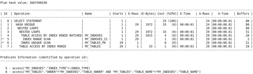
The LEADING hint specifies the order in which tables are processed, the INDEX hint specifies that an index be used, and the USE_NL hint specifies that tables be joined using the simple nested loop method (instead of the hash method used in previous executions). The use of the my_indexes_fk1 index reduces the number of consistent gets to 37.
Extreme Tuning
It does not appear possible to reduce consistent get operations any further because you are already using indexes to maximum advantage. Here is a summary of the previous execution strategy:
- Using the my_indexes_i1 index, collect the addresses of rows of the my_indexes table that qualify for inclusion.
- Using the addresses obtained in the previous step, retrieve the qualifying rows from the my_indexes table. There are 29 rows that qualify, and, therefore, you have to perform this step 29 times.
- For every qualifying row retrieved from the my_indexes table, use the my_tables_pk index and obtain the address of the matching row in the my_tables table. Obviously, 29 rows qualify.
- Using the addresses obtained in the previous step, retrieve the 29 matching rows from the my_tables table.
- Eliminate duplicates from the result.
It may appear that you have tuned the SQL statement as much as you can. However, there is a way to retrieve records quickly without the use of indexes, and there is a way to retrieve data from two tables without actually visiting two tables. Hash clusters allow data to be retrieved without the use of indexes; Oracle computes the hash signature of the record you need and translates the hash signature into the address of the record. Clustering effects can also significantly reduce the number of blocks that need to be visited to retrieve the required data. Further, materialized views combine the data from multiple tables and enable you to retrieve data from multiple tables without visiting the tables themselves. You can combine hash clusters and materialized views to achieve a dramatic reduction in the number of consistent get operations; in fact, you need only one consistent get operation.
First you create a hash cluster, and then you combine the data from my_tables and my_indexes into another table called my_tables_and_indexes. In the interests of brevity, you select only those items of information required by the query—items of information that would help other queries would normally be considered for inclusion:
PDB1@ORCL> CREATE CLUSTER my_cluster (index_type VARCHAR2(27)) SIZE 8192 HASHKEYS 5;

Cluster created.

PDB1@ORCL> CREATE MATERIALIZED VIEW LOG ON my_tables WITH ROWID;

Materialized view log created.
Next, you create a materialized view of the data. You use materialized view logs to ensure that any future changes to the data in my_tables or my_indexes are immediately made to the copy of the data in the materialized view. You enable query rewrite to ensure that your query is automatically modified and that the required data is retrieved from the materialized view instead of from my_tables and my_indexes. Appropriate indexes that would improve the usability and maintainability of the materialized view should also be created; I leave this as an exercise for you:
PDB1@ORCL> CREATE MATERIALIZED VIEW LOG ON my_indexes WITH ROWID;

Materialized view log created.

PDB1@ORCL> CREATE MATERIALIZED VIEW my_mv
  2  CLUSTER my_cluster (index_type)
  3  REFRESH FAST ON COMMIT
  4  ENABLE QUERY REWRITE
  5  AS
  6  SELECT t.ROWID AS table_rowid,
  7    t.owner AS table_owner,
  8    t.table_name,
  9    t.tablespace:name,
 10    i.ROWID AS index_rowid,
 11    i.index_type
 12  FROM my_tables t,
 13    my_indexes i
 14  WHERE t.owner = i.table_owner
 15  AND t.table_name = i.table_name;

Materialized view created.

PDB1@ORCL> EXEC DBMS_STATS.gather_table_stats(user, tabname=>’MY_MV’);

PL/SQL procedure successfully completed.

PDB1@ORCL> SELECT DISTINCT my_tables.owner,
  2    my_tables.table_name,
  3    my_tables.tablespace:name
  4  FROM my_tables,
  5    my_indexes
  6  WHERE my_tables.owner     = my_indexes.table_owner
  7  AND my_tables.table_name  = my_indexes.table_name
  8  AND my_indexes.index_type = :index_type;
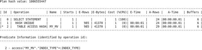
It’s now time to test the query again. You find that the number of consistent gets has been reduced to 6.
But Wait, There’s More!
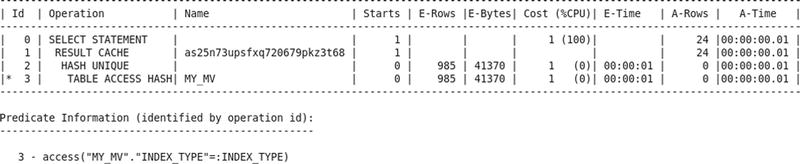
Executing a query obviously requires at least one consistent get operation. However, there is no need to execute the query if the query results have been previously cached and the data has not changed. Oracle 11g introduced the RESULT_CACHE hint to indicate that the data should be obtained from cache if possible. Note that this feature is available only with the Enterprise Edition. In the following example, you can see that the number of consistent gets has been reduced to zero!
PDB1@ORCL> SELECT /*+ RESULT_CACHE
  2    */
  3    DISTINCT my_tables.owner,
  4    my_tables.table_name,
  5    my_tables.tablespace:name
  6  FROM my_tables,
  7    my_indexes
  8  WHERE my_tables.owner     = my_indexes.table_owner
  9  AND my_tables.table_name  = my_indexes.table_name
 10  AND my_indexes.index_type = :index_type;

Statistics
----------------------------------------------------------
          0  recursive calls
          0  db block gets
          0  consistent gets
          0  physical reads
          0  redo size
       1751  bytes sent via SQL*Net to client
        554  bytes received via SQL*Net from client
          3  SQL*Net roundtrips to/from client
          0  sorts (memory)
          0  sorts (disk)
         24  rows processed
You saw four query plans in this exercise:
- The first query plan did not use any indexes because none had been created at the time.
- Qualifying records in my_indexes were efficiently identified by using the index on the values of index_type and were placed in a lookup table. All the records in my_tables were then retrieved and compared with the records in the lookup table.
- Qualifying records in my_indexes were efficiently identified using the index on the values of index_type. An index on the values of table_owner and table_name was then used to efficiently find the corresponding records in my_tables.
- A materialized view was used to combine the data from my_tables and my_indexes, and a hash cluster was used to create clusters of related records.
Summary
Here is a short summary of the concepts touched on in this chapter:
- The efficiency of an SQL statement is measured by the amount of computing resources used in producing the output. The number of logical read operations is a good way to measure the consumption of computing resources because it is directly proportional to the amount of resources consumed.
- Inefficient SQL can be identified by using tools such as Enterprise Manager and Toad, by tracing a batch job or user session, and by examining Statspack reports.
- Common causes for inefficient SQL are as follows: failure to use advanced features such as analytic functions, poor application development practices, poor logical and physical database design, and inadequate database maintenance.
- Hardware limitations and contention for limited resources play a major role in performance.
- The primary key of a table is always indexed. Indexes should be created on foreign keys unless the tables in question are small enough that the lack of an index will not have an impact on performance. Indexes should also be created on data items that are restricted in SQL queries. The dba_indexes and dba_ind_columns views show what indexes have been created. Most indexes are of the b*tree type. Other types of indexes are reverse key indexes, function-based indexes, and bitmap indexes. Clusters, index-organized tables, and table partitions are other options available to the database designer.
- Hints for the optimizer can be embedded in an SQL statement. Each hint partially constrains the optimizer, and a full set of hints completely constrains the optimizer. A desirable query plan can be preserved by capturing the set of hints that describes it in a stored outline.
- Statistical information on tables and indexes and the data they contain is what the query optimizer needs to do its job properly. Table and index statistics are automatically collected by a job called GATHER_STATS_JOB that runs during a nightly maintenance window. The DBMS_STATS package contains a variety of procedures for customizing the statistics collection strategy. System statistics are not collected automatically; they should be manually collected using the GATHER_SYSTEM_STATS procedure.
- One of the principal objectives of query tuning is to reduce the number of consistent get operations (logical reads) required. The theoretical lower bound on the number of consistent get operations is 1.
- The cost of creating a query plan can far exceed the cost of executing a query. Plan reuse is therefore critical for database performance. Dynamic sampling, necessitated by the absence of statistics, can dramatically increase the cost of creating a query plan.
- If you are using the Enterprise Edition and have a license for the Tuning Pack, you can use SQL Tuning Advisor to help you with SQL tuning.
Exercises
- Enable tracing of your SQL query by using the dbms_monitor.session_trace:enable and dbms_monitor.session_trace:disable procedures. Locate the trace file, and review the recursive calls. Also review the PARSE, EXECUTE, and FETCH calls for your query.
- Re-create the my_tables_and_indexes materialized view with all the columns in my_indexes and my_tables instead of just those columns required in the exercise. Does the materialized view need any indexes?
- Insert new data into my_tables and my_indexes, and verify that the data is automatically inserted into the materialized view.
Footnotes
1In Oracle on VMware, Dr. Bert Scalzo makes a persuasive case for “solving” problems with hardware upgrades: “Person hours cost so much more now than computer hardware even with inexpensive offshore outsourcing. It is now considered a sound business decision these days to throw cheap hardware at problems”.
2Don Burleson, “Optimizing Oracle Optimizer Statistics,” Oracle FAQ’s, March 1, 2004, www.orafaq.com/node/9.
3Mogens Norgaard in the Journal of the Northern California Oracle Users Group.
4Dave Ensor as remembered by Mogens Norgaard and quoted in the Journal of the Northern California Oracle Users Group.
5Mogens Norgaard in the Journal of the Northern California Oracle Users Group.
6Wolfgang Breitling in the Journal of the Northern California Oracle Users Group.
7Jonathan Lewis in the Journal of Northern California Oracle Users Group.
8The use of hints is a defense against bind variable peeking. To understand the problem, remember that a query-execution plan is constructed once and used many times. If the values of the bind variables in the first invocation of the query are not particularly representative of the data, the query plan that is generated will not be a good candidate for reuse. Stored outlines are another defense against bind variable peeking. It is also possible to turn off bind variable peeking for your session or for the entire database; this forces Oracle to generate a query plan that is not tailored to one set of bind variables. However, note that bind variable peeking does work well when the data has a uniform distribution.