
![]()
Numbers, Operators, Variables and Functions
Numbers
The numerical scope of MATLAB is very wide. Integer, rational, real and complex numbers, which in turn can be arguments of functions giving rise to whole, rational, real and complex functions. Therefore, the complex variable is a treatable field in MATLAB. This chapter will look at the basic functionality of MATLAB.
Arithmetic operations in MATLAB are defined according to the standard mathematical conventions. The following table presents the syntax of basic arithmetic operations:
|
x + y |
Sum >> 4 + 8 Ans = 12 |
|
x - y |
Difference >> 4 - 8 Ans = -4 |
|
x * y or x y |
Product >> 4 * 8 Ans = 32 |
|
x/y |
Division >> 4/8 Ans = 0.5000 |
|
x ^ y |
Power >> 4 ^ 8 Ans = 65536 |
MATLAB performs arithmetic operations as if it were a conventional calculator, but with total precision in the calculation. The results of operations presented are accurate for the default or for the degree of precision that the user prescribes. But this only affects the presentation. The feature that differentiates MATLAB from other numerical calculation programs in which the word length of the computer determines the accuracy, is that the calculation accuracy is unlimited in the case of MATLAB. MATLAB can represent the results with the accuracy that is required, although internally it always works with exact calculations to avoid rounding errors. MATLAB offers different approximate representation formats, which sometimes facilitate the interpretation of the results.
The following are the commands relating to the presentation of the results:
|
short format |
It offers results with 4 decimal. It’s the format default of MATLAB >> sqrt(23) ans = 4.7958 |
|
long format |
It delivers results with 16 decimal places >> format long; sqrt(23) Ans = 4.795831523312719 |
|
format long e |
Provides the results to 16 decimal places using the power of 10 >> format long e; SQRT (23) Ans = 4.795831523312719e + 000 |
|
format short e |
Provides the results to four decimal places with the power of 10 >> format short e; SQRT (23) Ans = 4.7958e + 000 |
|
format long g |
It offers results in optimal long format >> format long g; SQRT (23) Ans = 4.79583152331272 |
|
format short g |
It offers results in optimum short format >> format short g; SQRT (23) Ans = 4.7958 |
|
bank format |
It delivers results with 2 decimal places >> bank format; SQRT (23) Ans = 4.80 |
|
format rat |
It offers the results in the form of a rational number approximation >> format rat; SQRT (23) Ans = 1151/240 |
|
format + |
Offers a binary result using the sign (+, -) and ignores the imaginary part of the complex numbers >> format +; sqrt(23) Ans = + |
|
format hex |
It offers results in hexadecimal system >> format hex; sqrt(23) ans = 40132eee75770416 |
|
VPA ‘operations’ n |
It provides the result of operations with n exact decimal digits >> vpa 'sqrt(23)' 20 ans = 4.7958315233127195416 |
Integers and Integer Variable Functions
MATLAB works with integers and exact integer variable functions. Regardless of the format of presentation of the results, calculations are exact. Anyway, the command vpa allows exact outputs with the precision required.
In terms of functions with integer variables, the most important thing that MATLAB includes are as follows (the expressions between quotation marks have format string):
|
rem (n, m) |
Remainder of the division of n by m (valid function for n and m-real) >> rem(15,2) ans = 1 |
|
sign (n) |
Sign of n (1 if n > 0; -1 if n < 0) >> sign(-8) ans = -1 |
|
max (n1, n2) |
Maximum of the numbers n1 and n2 >> max(17,12) ans = 17 |
|
min (n1, n2) |
Minimum of the numbers n1 and n2 >> min(17,12) ans = 12 |
|
gcd (n1, n2) |
Greatest common divisor of n1 and n2 >> gcd(17,12) ans = 1 |
|
lcm (n1, n2) |
Least common multiple of n1 and n2 >> lcm(17,12) ans = 204 |
|
factorial (n) |
N factorial (n(n-1) (n-2)...)1) >> factorial(9) ans = 362880 |
|
factor (n) |
It decomposes the factorization of n >> factor(51) ans = 3 17 |
|
dec2base (decimal, n_base) |
Converts a specified decimal (base-10) number to the new base given by n_base >> dec2base(2345,7) ans = 6560 |
|
base2dec(numero,b) |
Converts the given base b number to a decimal number >> base2dec('ab12579',12) ans = 32621997 |
|
dec2bin (decimal) |
Converts a specified decimal number to base 2 (binary) >> dec2bin(213) ans = 11010101 |
|
dec2hex (decimal) |
Converts the specified decimal number to a base 16 (hexadecimal) number >> dec2hex(213) ans = D5 |
|
bin2dec (binary) |
Converts the binary number to a decimal based number >> bin2dec('1110001') ans = 113 |
|
hex2dec (hexadecimal) |
It converts the specified base 16 number to decimal >> hex2dec('FFAA23') ans = 16755235 |
Real Numbers and Functions of Real Variables
A rational number is of the form p/q, where p is an integer and q another integer. The way in which MATLAB processes rationals is different from that of the majority of calculators. The rational numbers are ratios of integers, and MATLAB also can work with them so that the result of expressions involving rational numbers is always another rational or whole number. So, it is necessary to activate this format with the command format rat. But MATLAB also returns solutions with decimals as the result if the user so wishes by activating any other type of format (e.g. format short or long format). We consider the following example:
>> format rat;
>> 1/6 + 1/5-2/10

Ans =

       1/6
MATLAB deals with rationals as ratios of integers and keeps them in this form during the calculations. In this way, rounding errors are not dragged into calculations with fractions, which can become very serious, as evidenced by the theory of errors. Once enabled in the rational format, operations with rationals will be exact until another different format is enabled. When the rational format is enabled, a number in floating point, or a number with a decimal point is interpreted as exact and MATLAB is exact in how the rational expression is represented with the result in rational numbers. At the same time, if there is an irrational number in a rational expression, MATLAB retains the number in the rational form so that it presents the solution in the rational form. We consider the following examples:
>> format rat;
>> 2.64/25+4/100

Ans =

      91/625

<Note that this is the result of 66/625 + 25/625.>

>> 2.64/sqrt(25)+4/100

Ans =

      71/125

>> sqrt(2.64)/25+4/100

Ans =

     204/1943
MATLAB also works with the irrational numbers representing the results with greater accuracy or with the accuracy required by the user, bearing in mind that the irrational cannot be represented as exactly as the ratio of two integers. Below is an example.
>> sqrt (235)

Ans =

     15.3297
There are very typical real constants represented in MATLAB as follows:
|
pi |
Number π = 3.1415926 >> 2 * pi Ans = 6.2832 |
|
exp (1) |
Number e = 2.7182818 >> exp (1) Ans = 2.7183 |
|
inf |
Infinity (for example 1/0) >> 1/0 Ans = INF |
|
nan |
Uncertainty (for example 0/0) >> 0/0 Ans = NaN |
|
realmin |
Least usable positive real number >> realmin Ans = 2.2251e-308 |
|
realmax |
Largest usable positive real number >> realmax Ans = 1.7977e + 308 |
MATLAB has a range of predefined functions of real variables.The following sectionss present the most important.
Trigonometric Functions
Below is a table with the trigonometric functions and their inverses that are incorporated in MATLAB illustrated with examples.
|
Function |
Inverse |
|---|---|
|
sin (x) sine >> sin(pi/2) ans = 1 |
asin (x) arcsine >> asin (1) ans = 1.5708 |
|
cos (x) cosine >> cos (pi) ans = -1 |
acos (x) arccosine >> acos (- 1) ans = 3.1416 |
|
tan(x) tangent >> tan(pi/4) ans = 1.0000 |
atan(x) atan2 (x) and arctangent >> atan (1) ans = 0.7854 |
|
csc(x) cosecant >> csc(pi/2) ans = 1 |
acsc (x) arccosecant >> acsc (1) ans = 1.5708 |
|
sec (x) secant >> sec (pi) ans = -1 |
asec (x) arcsecant >> asec (- 1) ans = 3.1416 |
|
cot (x) cotangent >> cot(pi/4) ans = 1.0000 |
acot (x) arccotangent >> acot (1) ans = 0.7854 |
Hyperbolic Functions
Below is a table with the hyperbolic functions and their inverses that are incorporated in MATLAB illustrated with examples.
|
Function |
Reverse |
|---|---|
|
sinh (x) hyperbolic sine >> sinh (2) ans = 3.6269 |
asinh (x) hyperbolic arcsine >> asinh (3.6269) ans = 2.0000 |
|
cosh(x) hyperbolic cosine >> cosh (3) ans = 10.0677 |
acosh(x) hyperbolic arccosine >> acosh (10.0677) ans = 3.0000 |
|
tanh(x) hyperbolic tangent >> tanh (1) ans = 0.7616 |
atanh (x) hyperbolic arctangent >> atanh (0.7616) ans = 1.0000 |
|
csch (x) hyperbolic cosecant >> csch (3.14159) ans = 0.0866 |
acsch (x) hyperbolic arccosecant >> acsch (0.0866) ans = 3.1415 |
|
sech (x) hyperbolic secant >> sech (2.7182818) ans = 0.1314 |
asech (x) hyperbolic arcsecant >> asech (0.1314) ans = 2.7183 |
|
coth (x) hyperbolic cotangent >> coth (9) ans = 1.0000 |
acoth (x) hyperbolic arccotangent >> acoth (0.9999) ans = 4.9517 + 1.5708i |
Exponential and Logarithmic Functions
Below is a table with the exponential and logarithmic functions that are incorporated in MATLAB illustrated with examples.
|
Function |
Meaning |
|---|---|
|
exp (x) |
Exponential function in base e (e ^ x) >> exp (log (7)) Ans = 7 |
|
log (x) |
Logarithmic function base e of x >> log (exp (7)) Ans = 7 |
|
log10 (x) |
Base 10 logarithmic function >> log10 (1000) Ans = 3 |
|
log2 (x) |
Logarithmic function of base 2 >> log2(2^8) Ans = 8 |
|
pow2 (x) |
Power function base 2 >> pow2 (log2 (8)) Ans = 8 |
|
sqrt (x) |
Function for the square root of x >> sqrt(2^8) Ans = 16 |
Numeric Variable-Specific Functions
MATLAB incorporates a group of functions of numerical variable. Among these features are the following:
|
Function |
Meaning |
|---|---|
|
abs (x) |
Absolute value of the real x >> abs (- 8) Ans = 8 |
|
floor (x) |
The largest integer less than or equal to the real x >> floor (- 23.557) Ans = -24 |
|
ceil (x) |
The smallest integer greater than or equal to the real x >> ceil (- 23.557) Ans = -23 |
|
round (x) |
The closest integer to the real x >> round (- 23.557) Ans = -24 |
|
fix (x) |
Eliminates the decimal part of the real x >> fix (- 23.557) Ans = -23 |
|
rem (a, b) |
It gives the remainder of the division between the real a and b >> rem (7.3) Ans = 1 |
|
sign (x) |
The sign of the real x (1 if x > 0; - 1 if x < 0) >> sign (- 23.557) Ans = -1 |
One-Dimensional, Vector and Matrix Variables
MATLAB is software based on matrix language, and therefore focuses especially on tasks for working with arrays.
The initial way of defining a variable is very simple. Simply use the following syntax:
Variable = object
where the object can be a scalar, a vector or a matrix.
If the variable is an array, its syntax depends on its components and can be written in one of the following ways:
Variable = [v1 v2 v3... vn]
Variable = [v1, v2, v3,..., vn]
If the variable is an array, its syntax depends on its components and can be written in one of the following ways:
Variable = [v11 v12 v13... v1n; v21 v22 v23... v2n;...]
Variable = [v11, v12, v13,..., v1n; v21, v22, v23,..., v2n;...]
Script variables are defined in the command window from MATLAB in a natural way as shown in Figure 2-1.
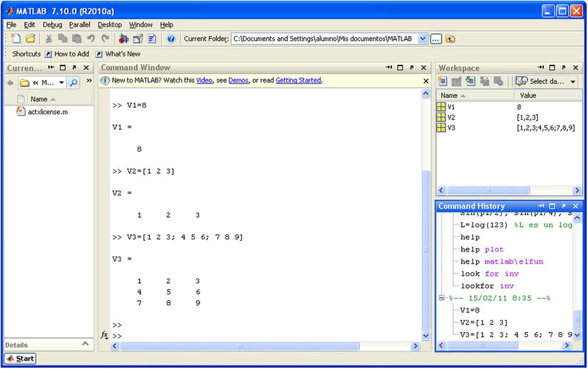
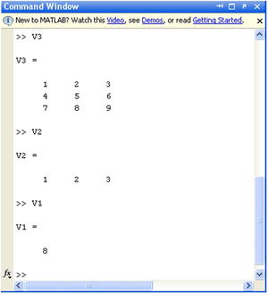
The workspace (Workspace) window contains all variables that we will define in the session. The value of any of these variables is recoverable by typing their names on the command window (Figure 2-2).
Also, in the command history window (Command History) we can find all the syntax we execute from the command window.
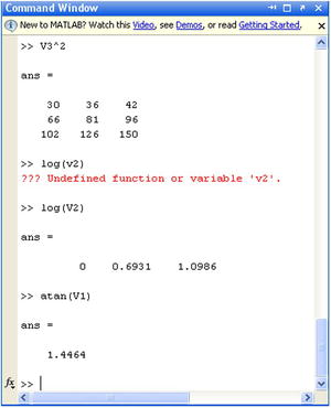
Once a variable is defined, we can operate on it using it as a regular variable in mathematics, bearing in mind that the names of the variables are sensitive to upper and lower case. Figure 2-3 shows some operations with one-dimensional, vector and matrix variables. It is important to note the error that occurred when calculating the logarithm of V2. The mistake was changing the variable to lowercase so that it was not recognized.
MATLAB variables names begin with a letter followed by any number of letters, digits or underscores with a 31 character maximum.
There are also specific forms for the definition of vector variables, among which are the following:
|
variable = [a: b] |
Defines the vector whose first and last elements are a and b, respectively, and the intermediate elements differ by one unit >> vector1 = [2:6] vector1 = 2 3 4 5 6 |
|
variable = [a: s:b] |
Defines the vector whose first and last elements are a and b, and the intermediate elements differ in the amount specified by the increase in s >> vector2 = [2:2:8] Vector2 = 2 4 6 8 |
|
Nvariable = linespace [a, b, n] |
Defines the vector whose first and last elements are a and b, and has in total n evenly spaced elements >> vector3 = linespace (10,30,6) Vector3 = 10 14 18 22 26 30 |
Elements of Vector Variables
MATLAB allows the selection of elements of vector variables using the following commands:
|
x (n) |
Returns the nth element of the vector x >> X =(2:8) X = 2 3 4 5 6 7 8 >> X (3) Ans = 4 |
|
x(a:b) |
Returns the elements of the vector x between the a-th and the b-th elements, both inclusive >> X (3:5) Ans = 4 5 6 |
|
x(a:p:b) |
Returns the elements of the vector x located between the a-th and the b-th elements, both inclusive, but separated by units where a < b. >> X (1:2:6) Ans = 2-4-6 |
|
x(b:-p:a) |
Returns the elements of the vector x located between the b- and a-th, both inclusive, but separates by p units and starting with the b-th element (b > a) >> X(6:-2:1) Ans = 7-5-3 |
Elements of Matrix Variables
The same as in the case of vectors, MATLAB allows the selection of elements of array variables using the following commands:
|
A(m,n) |
Defines the (m, n) element of the matrix A (row m and column n) >> A = [3 5 7 4; 1 6 8 9; 2 6 8 1] A = 3 5 7 4 1 6 8 9 2 6 8 1 >> A (2,4) Ans = 9 |
|
A(a:b,c:d) |
Defines the subarray of A formed by the intersection of the a-th and the b-th rows and the the c-th and the d-th columns >> A(1:2,2:3) Ans = 5 7 6 8 |
|
A(a:p:b,c:q:d) |
Defines the subarray of A formed by rows between the a-th and the b-th spaced by using p in p, and the columns between the c-th and the d-th spaced by using q in q >> A(1:2:3,1:2:4) Ans = 3 7 2 8 |
|
A([a b],[c d]) |
Defines the subarray of A formed by the intersection of the a-th and b-th rows and c-th and d-th columns >> A([2 3],[2 4]) Ans = 6 9 6 1 |
|
A([a b c...],) ([e f g...]) |
Defines the subarray of A formed by the intersection of rows a, b, c,... and columns e, f, g,... >> A([2 3],[1 2 4]) Ans = 1-6-9 2-6-1 |
|
A(:,c:d) |
Defines the subarray of A formed by all the rows from A and columns between the c-th and the d-th >> A(:,2:4) Ans = 5 7 4 6 8 9 6 8 1 |
|
A(:,[c d e...]) |
Defines the subarray of A formed by all the rows from A and columns c, d, e,... >> A(:,[2,3]) Ans = 5 7 6 8 6 8 |
|
A(a:b,:) |
Defines the subarray of A formed by all the columns in A and rows between the a-th and the b-th >> A(2:3,:) Ans = 1 6 8 9 2 6 8 1 |
|
A([a b c...],:) |
Defines the subarray of A formed by all the columns in A and rows a, b, c,... >> A([1,3],:) Ans = 3 5 7 4 2 6 8 1 |
|
A(a,:) |
Defines the a-th row of the matrix A >> A(3,:) Ans = 2 6 8 1 |
|
A(:,b) |
Defines the b-th column of the matrix A >> A(:,3) Ans = 7 8 8 |
|
A (:) |
Defines a vector column whose elements are the columns of A placed order one below another >> A (:) Ans = 3 1 2 5 6 6 7 8 8 4 9 1 |
|
A(:,:) |
It is equivalent to the matrix A >> A(:,:) Ans = 3 5 7 4 1 6 8 9 2 6 8 1 |
|
[A, B, C,...] |
Defines the matrix formed by the subarrays A, B, C,... >> A1 = [2 6; 4 1], A2 = [3 8; 6 9] A1 = 2 6 4 1 A2 = 3 8 6 9 >> [A1, A2] Ans = 2 6 3 8 4 1 6 9 |
Specific Matrix Functions
MATLAB uses a group of predefined matrix functions that facilitate the work in the matrix field. The most important are the following:
|
diag (v) |
Create a diagonal matrix with the vector v in the diagonal >> diag([2 0 9 8 7]) Ans = 2 0 0 0 0 0 0 0 0 0 0 0 9 0 0 0 0 0 8 0 0 0 0 0 7 |
|
diag (A) |
Extract the diagonal of the matrix as a vector column >> A = [1, 3, 5; 2 0 8; -1-3 2] A = 1 3 5 2 0 8 -1-3 2 >> diag (A) Ans = 1 0 2 |
|
eye (n) |
It creates the identity matrix of order n >> eye (4) Ans = 1 0 0 0 0 1 0 0 0 0 1 0 0 0 0 1 |
|
eye (m, n) |
Create order mxn matrix with ones on the main diagonal and zeros elsewhere >> eye (3.5) Ans = 1 0 0 0 0 0 1 0 0 0 0 0 1 0 0 |
|
zeros (m, n) |
Create the zero matrix of order m x n >> zeros (2,3) Ans = 0 0 0 0 0 0 |
|
ones (m, n) |
Create the matrix of order with all its elements 1 m x n >> ones (2,3) Ans = 1 1 1 1 1 1 |
|
rand (m, n) |
It creates a uniform random matrix of order m x n >> rand (4.5) Ans = 0.8147 0.6324 0.9575 0.9572 0.4218 0.9058 0.0975 0.9649 0.4854 0.9157 0.1270 0.2785 0.1576 0.8003 0.7922 0.9134 0.5469 0.9706 0.1419 0.9595 |
|
randn (m, n) |
Create a normal random matrix of order m x n >> randn (4.5) Ans = 0.6715 0.4889 0.2939 - 1.0689 0.3252 -1.2075 1.0347 - 0.7873 - 0.8095 - 0.7549 0.7172 0.7269 0.8884 - 2.9443 1.3703 1.6302 - 0.3034 - 1.1471 1.4384 - 1.7115 |
|
flipud (A) |
Returns the matrix whose rows are placed in reverse order (from top to bottom) to the rows of matrix A >> flipud (A) Ans = -1-3 2 2 0 8 1 3 5 |
|
fliplr (A) |
Returns the matrix whose columns are placed in reverse (from left to right) of A >> fliplr (A) Ans = 5 3 1 8 0 2 2-3-1 |
|
rot90 (A) |
Rotates 90 degrees the matrix A >> rot90 (A) Ans = 5 8 2 3 0-3 1 2-1 |
|
reshape(A,m,n) |
Returns the array of order extracted from matrix m x n taking consecutive items by columns >> reshape(A,3,3) Ans = 1 3 5 2 0 8 -1-3 2 |
|
size (A) |
Returns the order (size) of the matrix A >> size (A) Ans = 3 3 |
|
length (v) |
Returns the length of the vector v >> length([1 3 4 5-1]) Ans = 5 |
|
tril (A) |
Returns the lower triangular part of matrix A >> tril (A) Ans = 1 0 0 2 0 0 -1-3 2 |
|
triu (A) |
Returns the upper triangular part of matrix A >> (A) triu Ans = 1 3 5 0 0 8 0 0 2 |
|
A’ |
Returns the transposed matrix from A >> A' Ans = 1 2-1 3 0-3 5 8 2 |
|
Inv (A) |
Returns the inverse matrix of matrix A >> inv(A) Ans = -0.5714 0.5000 - 0.5714 0.2857 - 0.1667 - 0.0476 0.1429 0.1429 0 |
Random Numbers
MATLAB incorporates features that make it possible to work with randomised numbers. The functions rand and randn are basic functions that generate random numbers distributed uniformly and normally respectively. Below are the most common functions for working with random numbers.
|
rand |
Returns a random decimal number uniformly distributed in the interval [0,1] >> rand Ans = 0.8147 |
|
rand (n) |
Returns an array of size n x n whose elements are uniformly distributed random decimal numbers in the interval [0,1] >> rand (3) Ans = 0.9058 0.6324 0.5469 0.1270 0.0975 0.9575 0.9134 0.2785 0.9649 |
|
rand (m, n) |
Returns an array of dimension m x n whose elements are uniformly distributed random decimal numbers in the interval [0,1] >> rand (2,3) Ans = 0.1576 0.9572 0.8003 0.9706 0.4854 0.1419 |
|
rand (size (a)) |
Returns an array of the same size as the matrix A and whose elements are uniformly distributed random decimal numbers in the interval [0,1] >> rand (size (eye (3))) Ans = 0.4218 0.9595 0.8491 0.9157 0.6557 0.9340 0.7922 0.0357 0.6787 |
|
rand (‘seed’) |
Returns the current value of the uniform random number generator seed >> rand('seed') Ans = 931316785 |
|
rand(‘seed’,n) |
Placed in the number n, the current value of the uniform random number generator seed >> rand ('seed') Ans = 931316785 >> rand ('seed', 1000) >> rand ('seed') Ans = 1000 |
|
randn |
Returns a random decimal distributed number according to a normal distribution of mean 0 and variance 1 >> randn Ans = -0.4326 |
|
randn (n) |
Returns an array of size n x n whose elements are distributed random decimal numbers according to a normal distribution of mean 0 and variance 1 >> randn (3) Ans = -1.6656 - 1.1465 - 0.0376 0.1253 1.1909 0.3273 0.2877 1.1892 0.1746 |
|
randn (m, n) |
Returns an array of dimension m x n whose elements are distributed random decimal numbers according to a normal distribution of mean 0 and variance 1 >> randn (2,3) Ans = -0.1867 - 0.5883 - 0.1364 0.7258 2.1832 0.1139 |
|
randn (size (A)) |
Returns an array of the same size as the matrix A and whose elements are distributed according to a normal distribution of mean 0 and variance 1 as random decimal numbers >> randn (size (eye (3))) Ans = 1.0668 - 0.8323 0.7143 0.0593 0.2944 1.6236 -0.0956 - 1.3362 - 0.6918 |
|
randn (‘seed’) |
Returns the current value of the normal random number generator seed >> randn ('seed') Ans = 931316785 |
|
randn(‘seed’,n) |
Placed in the n number the current value of the uniform random number generator seed >> randn ('seed', 1000) >> randn ('seed') Ans = 1000 |
Operators
MATLAB is a language that incorporates arithmetic, logical and relational operators in the same way as any other language. The following are the types of operators referred to in the scope of the MATLAB language.
Arithmetic Operators
MATLAB incorporates the usual arithmetic operators (addition, subtraction, multiplication and division) to work with numbers. MATLAB extends the meaning of these operators to work with scalars, vectors and matrices, as shown in the following table:
|
Operator |
Role Played |
|---|---|
|
+ |
Sum of scalar, vector, or matrix >> A = [1 3 -2 6]; B = [4 -5 8 2]; c = 3; >> V1 = A + c V1 = 4 6 1 9 >> V2 = A + B V2 = 5 –2 6 8 |
|
- |
Subtraction of scalar, vector, or matrix >> V3 = A-c V3 = -2 0 -5 3 >> V4 = A - B V4 = -3 8 -10 4 |
|
* |
Product of scalars or arrays or scalars vectors or matrices Defines the subarray of A formed by the intersection of the a-th and the b-th rows and the the c-th and the d-th columns >> V3 = A * c V3 = 3 9 -6 18 |
|
.* |
Product of scalar or vector element to element >> V4 = A * B V4 = 4 -15 -16 12 |
|
.^ |
Power of vectors (A. ^ B = [A(i,j)B (i, j)], vectors A and B) >> V6 = a ^ B V6 = 1.0000 0.0041 256.0000 36.0000 >> A ^ c Ans = 1 27 -8 216 >> c. ^ A Ans = 3.0000 27.0000 0.1111 729.0000 |
|
./ |
A / B = [A(i,j)/b (i, j)], being A and B vectors where [dim (A) = dim (B)] >> V7 = A. / B V7 = 0.2500 - 0.6000 - 0.2500 3.0000 |
|
. |
A. B = [B(i,j) /A (i, j)], being A and B vectors where [dim (A) = dim (B)] >> V8 = A. B V8 = 4.0000 - 1.6667 - 4.0000 0.3333 |
|
|
AB = inv (A) * B, with A and B being matrices >> A = rand (4) A = 0.6868 0.5269 0.7012 0.0475 0.5890 0.0920 0.9103 0.7361 0.9304 0.6539 0.7622 0.3282 0.8462 0.4160 0.2625 0.6326 >> B = randn (4) B = -0.1356 - 0.0449 - 0.0562 0.4005 -1.3493 - 0.7989 0.5135 - 1.3414 -1.2704 - 0.7652 0.3967 0.3750 0.9846 0.8617 0.7562 1.1252 >> AB Ans = 25.0843 17.5201 - 1.8497 7.1332 -25.8285 - 17.9297 2.4290 - 4.6114 -4.4616 - 3.1424 - 0.2409 - 2.7058 -13.1598 - 8.9778 2.1720 - 3.6075 |
|
/ |
Ratio scale of b/a = B * inv (A), with A and B being matrices >> B/A Ans = -4.8909 0.0743 4.8972 - 1.6273 4.6226 0.9230 - 4.2151 - 1.3541 -10.2745 1.2107 10.4001 - 5.4409 -9.6925 - 0.1247 11.1342 - 3.1260 |
|
^ |
Power of scalar or power scale matrix (M p) >> A ^ 3 Ans = 3.5152 2.1281 3.1710 1.6497 4.0584 2.3911 3.7435 1.9881 4.6929 2.8299 4.2067 2.2186 3.5936 2.1520 3.2008 1.7187 |
Logical Operators
MATLAB also includes the usual logical operators using the most common notation for them. The results of the logical operators usually are 1 if true and or if false. These operators are shown in the following table.
|
~ A |
Logical negation (NOT) or A supplementary >> not(2 > 3) Ans = 1 |
|
A & B |
Logical conjunction (AND) or the intersection of A and B >> (2 > 3) & (5 > 1) Ans = 0 |
|
A | B |
Logical disjunction (OR) or the union of A and B >> (2 > 3) |(5 > 1) Ans = 1 |
|
XOR (A, B) |
OR exclusive (XOR) or symmetric difference of A and B (it’s true [1] if A or B is true, but not both) >> xor ((2 > 3),(5 > 1)) Ans = 1 |
Relational Operators
MATLAB also deals with relational operations that run comparisons element by element between two matrices, and returns an array of the same size whose elements are zero if the corresponding relationship is true, or one if the corresponding relation is false. The relational operators can also compare scalar vectors or matrices, in which case it is compared to climbing with all the elements of the array. The following table shows the relational operators in MATLAB.
|
< |
Lower (for complex it compares only the real parts) >> 3 < 5 Ans = 1 |
|
< = |
Less than or equal (only applies to real parts) >> 4 >= 6 Ans = 0 |
|
> |
Wholesale (only applies to real parts) >> X = 3 * ones (3.3) X = 3 3 3 3 3 3 3 3 3 >> X > [1 2 3; 4 5 6; 1 2 3] Ans = 1 1 0 0 0 0 1 1 0 |
|
> = |
Greater than or equal (only applies to real parts) >> X >= [1 2 3; 4 5 6; 1 2 3] Ans = 1 1 1 0 0 0 1 1 1 |
|
x == y |
Equality (affects complex numbers) >> X == ones (3,3) Ans = 0 0 0 0 0 0 0 0 0 |
|
x ~ = y |
Inequality (affects complex numbers) >> X ~= ones (3,3) Ans = 1 1 1 1 1 1 1 1 1 |
Symbolic Variables
So far we have always handled numerical variables. However, MATLAB allows you to manage symbolic mathematical computation, manipulating formulae and algebraic expressions easily and quickly and perform operations with them.
However, to accomplish these tasks it is necessary to have the MATLAB Symbolic Math Toolbox module. Algebraic expressions or variables to be symbolic have to be declared as such with the command syms, before they are used. The following table shows the command syntax of conversion variables and symbolic expressions.
|
syms x y z... t |
Converts the variables x, y and z,..., t into symbolic >> syms x y >> x+x+y-6*y Ans = 2 * x - 5 * y |
|
syms x y z... t real |
Converts the variables x, y and z,..., t into symbolic with actual values >> syms a b c real; >> A = [a b c; c a b; b c a] A = [a, b, c] [c, a, b] [b, c, a] |
|
syms x and z... t unreal |
Converts the variables x, y and z,..., t into symbolic with no actual values |
|
syms |
Symbolic workspace variables list >> syms 'A' 'a' 'ans' 'b' 'c' 'x' 'y' |
|
y = sym (‘x’) |
Converts the variable or number x in symbolic (equivalent to syms x) >> rho = sym ('(1 + sqrt (5)) / 2') Rho = 5 ^(1/2)/2 + 1/2 |
|
y = sym (‘x’, real) |
It becomes a real symbolic variable x |
|
y = sym(‘x’, unreal) |
It becomes a non-real symbolic variable x |
|
S = sym (A) |
Creates a symbolic object starting with A, where A may be a string, a scalar, an array, a numeric expression, etc. >> S = sym([0.5 0.75 1; 0 0.5 0.1; 0.2 0.3 0.4]) S = [1/2, 3/4, 1] [ 0, 1/2, 1/10] [1/5, 3/10, 2/5] |
|
S = sym (at, ‘option’) |
Converts the array, scalar or a numeric expression to symbolic according to the specified option. The option can be ‘f’ for floating point, ‘r’ for rational, ‘e’ for error format and ‘d’ for decimal |
|
numeric(x) or double(x) |
It becomes the variable or expression x to numeric double-precision |
|
pretty (expr) |
Converts the symbolic expression to written mathematics >> pretty (rho) 1/2 5 1 ---- + - 2 2 |
|
Digits |
The current accuracy for symbolic variables >> digits Digits = 32 |
|
digits (d) |
The precision of symbolic variables in d exact decimal digits >> digits (25) >> digits Digits = 25 |
|
vpa (‘expr’) |
Numerical result of the expression with decimals of precision in digits >> phi = vpa ('(1 + sqrt (5)) / 2') Phi = 1.618033988749894848204587 |
|
vpa(‘expr’, n) |
Numerical results of the expression with n decimal digits >> phi = vpa ('(1 + sqrt (5)) / 2', 10) Phi = 1.618033989 |
|
vpa (expr, n) |
Numerical result of the expression with n decimal digits >> phi = vpa ((1 + sqrt (5)) / 2.20) Phi = 1.6180339887498949025 |
Symbolic Functions and Functional Operations: Composite and Inverse Functions
In MATLAB, it is possible to define functions to measure of one and several variables using the syntax f = ‘function’.
Also you can use the syntax f = function if all variables have been defined previously as symbolic with syms. Subsequently it is possible to make substitutions to your arguments according to the notation which is presented in the following table.
The results tend to simplify the commands simple and simplify.
|
f = ‘function’ |
It defines the function f as symbolic >> f1 ='x ^ 3' F1 = x ^ 3 >> f2 ='z ^ 2 + 2 * t' F2 = z ^ 2 + 2 * t >> syms x t z >> g1 = x ^ 2 G1 = x ^ 2 >> g2 = sqrt (x+2 * z + exp (t)) G2 = (x + 2 * z + exp (t)) ^(1/2) |
|
subs(f, a) |
Applies the function f at the point a >> subs(f1,2) Ans = 8 |
|
subs (f, variable, value) |
Replaces the variable by a value >> subs(f1,x,3) Ans = 27 |
|
subs(f, {x,y,...}, {a,b,...}) |
Replaces the variables in the equation f {x, y,..} with the values {a, b,...} >> subs(f2, {z,t}, {1,2}) Ans = 5 |
MATLAB additionally implements various functional operations which are summarized in the following table:
|
f + g |
Adds the functions f and g (f + g) >> syms x >> f = x ^ 2 + x + 1; g = 2 * x ^ 2-x ^ 3 + cos (x); h =-x+log (x); >> f + g Ans = x + cos (x) + 3 * x ^ 2 - x ^ 3 + 1 |
|
f+g+h+... |
Performs the sum f+g+h +... >> f+g+h Ans = cos (x) + log (x) + 3 * x ^ 2 - x ^ 3 + 1 |
|
f-g |
Find the difference of f and g (f-g) >> f-g Ans = x cos (x) - x ^ 2 + x ^ 3 + 1 |
|
f-g-h-... |
Performs the difference f-g-h-... >> f-g-h Ans = 2 * x - cos (x) - log (x) - x ^ 2 + x ^ 3 + 1 |
|
f * g |
Creates the product of f and g (f * g) >> f * g Ans = (cos (x) + 2 * x ^ 2 - x ^ 3) * (x^2 + x + 1) |
|
f*g*h*... |
Creates the product f * g * h *... >> f * g * h Ans = -(x - log (x)) * (cos (x) + 2 * x ^ 2 - x ^ 3) * (x^2 + x + 1) |
|
f/g |
Performs the ratio between f and g (f/g) >> f/g Ans = (x ^ 2 + x + 1) / (cos (x) + 2 * x ^ 2 - x ^ 3). |
|
f/g/h/... |
Performs the ratio f /g/h... >> f Ans = -(x^2 + x + 1) / ((x - log (x)) * (cos (x) + 2 * x ^ 2 - x ^ 3)) |
|
f ^ k |
Raises f to the power k (k is a scalar) >> f ^ 2 Ans = (x ^ 2 + x + 1) ^ 2 |
|
f ^ g |
It elevates a function to another function (fg) >> f ^ g Ans = (x ^ 2 + x + 1) ^ (cos (x) + 2 * x ^ 2 - x ^ 3). |
|
compose (f, g) |
A function of f and g (f ° g (x) = f (g (x))) >> compose (f, g) Ans = cos (x) + (cos (x) + 2 * x ^ 2 - x ^ 3) ^ 2 + 2 * x ^ 2 - x ^ 3 + 1 |
|
compose(f,g,h) |
Function of f and g, taking the expression or as the domain of f and g >> compose (f, g, h) Ans = cos (log (x) - x) + 2 * (x - log (x)) ^ 2 + (x - log (x)) ^ 3 + (cos (log (x) |
|
g = finverse (f) |
Inverse of the function f >> finverse (f) Warning: finverse(x^2 + x + 1) is not unique. Ans = (4 * x - 3) ^(1/2)/2 - 1/2 |
Commands that Handle Variables in the Workspace and Store them in Files
MATLAB has a group of commands that allow you to define and manage variables, as well as store them in MATLAB format files (with extension .mat) or in ASCII format, in a simple way. When extensive calculations are performed, it is convenient to give names to intermediate results. These intermediate results are assigned to variables to make it easier to use. Let’s not forget that the value assigned to a variable is permanent until it is expressly changed or is out of the present session of work. MATLAB incorporates a group of commands to manage variables among which are the following:
|
clear clear(v1,v2, ..., vn) clear(‘v1’, ‘v2’, ..., ‘vn’) |
Clears all variables in the workspace Deletes the specified numeric variables Clears the variables specified in a string |
|
disp(X) |
Shows an array without including its name |
|
length(X) |
Shows the length of the vector X and if X is an array, displays its greatest dimension |
|
load load file load file X Y Z load file -ascii load file -mat S = load(...) |
It reads all variables from the file MATLAB.mat Reads all variables specified as .mat files Reads the variables X, Y, Z of the given .mat file It reads the file as ASCII whatever its extension It reads the file as .mat whatever its extension Returns the contents of a file in the variable .mat S |
|
saveas(h,‘f.ext’) saveas(h,‘f’, ‘format’) |
Saves the figure or model h as a f.ext file Save the figure or model h as the f in the specified format file |
|
d = size(X) [m,n] = size(X) [d1,d2,d3,...,dn] = size(X) |
Returns the sizes of each dimension in a vector Returns the dimensions of the matrix X as two variables named m & n Returns the dimensions of the array X as variable names d1, d2,..., dn |
|
who whos who(‘-file’, ‘fichero’) whos(‘-file’, ‘fichero’) who(‘var1’, ‘var2’,...) who(‘-file’, ‘filename’, ‘var1’, ‘var2’,...) s = who(...) s = whos(...) who -file filename var1 var2 ... whos -file filename var1 var2 ... |
The variables in the workspace list List of variables in the workspace with your sizes and types List of variables in the given .mat file List of variables in the given .mat file and their sizes and types List of the variables string from the given workspace List of the variables specified in the string in the given .mat file The listed variables stored in s The variables with their sizes and types stored in s List of numerical variables specified in the given .mat file List of numerical variables specified in the file .mat given with their sizes and types |
|
Workspace |
Shows a browser to manage the workspace |
The save command is the essential instrument for storing data in the MATLAB .mat file type (only readable by the MATLAB program) and in file type ASCII (readable by any application). By default, the storage of variables often occurs in files formatted using MATLAB .mat. To store variables in files formatted in ASCII, it is necessary to use the command save with the options that are presented below:
|
Option |
Mode of storage of the data |
|---|---|
|
-append |
The variables are added to the end of the file |
|
-ascii |
The variables are stored in a file in ASCII format of 8 digits |
|
-ascii - double |
The variables are stored in a file in ASCII format of 16 digits |
|
-ascii – tabs |
The variables are stored in a tab-delimited file in ASCII format of 8 digits |
|
-ascii - double - tabs |
The variables are stored in a tab-delimited file in ASCII format of 16 digits |
|
-mat |
The variables are stored in a file with binary .mat format |
EXERCISE 2-1
Calculate the value of 7 to the 400th power with 500 exact decimal numbers.
>> vpa '7 ^ 400' 500
Ans =
3234476509624757991344647769100216810857201398904625400933895331391691459636928060001*10^338
500 figures are not needed to express the exact value of the result. It notes that it is enough with 338 figures. If you want the result with less accurate figures than it actually is, MATLAB completes the result with powers of 10. Let's see:
>> vpa '7 ^ 400' 45
Ans =
1.09450060433611308542425445648666217529975487 * 10 ^ 338
EXERCISE 2-2
Calculate the greatest common divisor and least common multiple of the numbers 1000, 500 and 625
>> gcd (gcd (1000,500), 625)
Ans =
125
As the gcd function only supports two arguments in MATLAB, we have applied the property: gcd(a, b, c) = gcd (gcd(a, b), c) = gcd(a, gcd (b, c)). The property is analogous to the least common multiple: lcm(a, b, c) = lcm (lcm(a, b), c) = lcm (a, lcm (b, c)). We will make the calculation in the following way:
>> lcm(lcm(1000,500), 625)
Ans =
5000
EXERCISE 2-3
Is the number 99,991 prime? Find the prime factors of the number 135,678,742.
We divide both numbers into prime factors:
>> factor (99991)
Ans =
99991
>> factor (135678742)
Ans =
2 1699 39929
It is observed that 99991 is a prime number because in attempting to break it down into prime factors, it turns out to be the only prime factor of itself. Observe that the number 135678742 has three prime factors.
EXERCISE 2-4
Find the remainder of dividing 2134 by 3. Is the number 232 – 1 divisible by 17? Also find the number N which divided by 16, 24, 30 and 32 yields a remainder of 5.
The first part of the problem is resolved as follows:
>> rem(2^134,3)
Ans =
0
It is observed that 2134 is a multiple of 3.
To see if 232 – 1 is divisible by 17, we factor it:
>> factor(2^32-1)
Ans =
3 5 17 257 65537
Note that 17 is one of its factors, so then it is divisible by 17.
To resolve the last part of the problem, we calculate the least common multiple of all the numbers and add 5.
>> N = 5+lcm(16,lcm(24,lcm(30,32)))
N =
485
EXERCISE 2-5
Calculate the value of 100 factorial. Calculate it also with 70 and 200 significant figures.
>> factorial(100)
ans =
9.3326e+157
>> vpa(factorial(100))
ans =
9.3326215443944102188325606108575*10^157
>> vpa(factorial(100),70)
ans =
9.3326215443944102188325606108575267240944254854960571509166910400408*10^157
>> vpa(factorial(100),200)
ans =
9.33262154439441021883256061085752672409442548549605715091669104004079950642429371486326
94030450512898042989296944474898258737204311236641477561877016501813248*10^157
EXERCISE 2-6
In base 5 the results of the following operation:
a25aaff6 + 6789aba + 1100221 + 35671 - 1250
16 12 8 3
As it is a venture to convert between numbers in different base numbering systems, it will be simplest to convert to base 10 first and then perform the operation to calculate the result in base-5.
>>R10=base2dec('a25aaf6',16)+base2dec('6789aba',12)+base2dec('35671',8) + base2dec('1100221',3)-1250
R10 =
190096544
>> R5 = dec2base (R10, 5)
R5 =
342131042134
EXERCISE 2-7
In base 13, get the result of the following operation:
(666551) (aa199800a) + (fffaaa125) / (33331 + 6)
7 11 16 4
We use the strategy of the previous exercise. First, we make the operation with all the numbers to base 10 and then find the result for base 13.
>> R10 = vpa (base2dec('666551',7) * base2dec('aa199800a',11) + 79 * base2dec('fffaaa125',16) / (base2dec ('33331', 4) + 6))
R10 =
275373340490851.53125
>> R13 = dec2base (275373340490852,13)
R13 =
BA867963C1496
EXERCISE 2-8
Perform the following operations with rational numbers:
a. 3/5 + 2/5 + 7/5
b. 1/2 + 1/3 + 1/4 + 1/5 + 1/6
c. 1/2-1/3 + 1/4 - 1/5 + 1/6
d. (2/3-1/6)-(4/5+2+1/3) + (4-5/7)
a.
>> format rat
>> 3/5 + 2/5 + 7/5
Ans =
12/5
b.
>> 1/2 + 1/3 + 1/4 + 1/5 + 1/6
Ans =
29/20
c.
>> 1/2-1/3 + 1/4 - 1/5 + 1/6
Ans =
23/60
d.
>> (2/3-1/6)-(4/5+2+1/3) + (4-5/7)
Ans =
137/210
Alternatively, also the operations can be made as follows:
>> simplify (sym(3/5+2/5+7/5))
Ans =
12/5
>> simplify (sym(1/2+1/3+1/4+1/5+1/6))
Ans =
29/20
>> simplify (sym(1/2-1/3+1/4-1/5+1/6))
Ans =
23/60
>> simplify (sym ((2/3-1/6)-(4/5+2+1/3) +(4-5/7)))
Ans =
137/210
EXERCISE 2-9
Perform the following rational operations:
a. 3/a+2/a+7/a
b. 1 / (2a) + 1 / (3a) + 1 / (4a) + 1 / (5a) + 1 / (6a)
c. 1 / (2a) + 1 / (3b + 1 / (4a) + 1 / (5b) + 1 / (6c))
To treat operations with expressions that contain symbolic variables a it is necessary to prepend the command syms a to declare the variable as symbolic, and then use simplify or simple.
a.
>> syms a
>> simplify(3/a+2/a+7/a)
Ans =
12/a
>> 3/a+2/a+7/a
Ans =
12/a
>> Ra = simple(3/a+2/a+7/a)
RA =
12/a
b.
>> simplify (1 /(2*a) + 1 /(3*a) + 1 /(4*a) + 1 /(5*a) + 1 /(6*a))
Ans =
29 /(20*a)
>> Rb = simple (1 /(2*a) + 1 /(3*a) + 1 /(4*a) + 1 /(5*a) + 1 /(6*a))
RB =
29 /(20*a)
c.
>> syms a b c
>> pretty (simplify (1 /(2*a) + 1 /(3*b) + 1 /(4*a) + 1 /(5*b) + 1 /(6*c)))
3 8 1
--- + ---- + --
4a 15b 6c
>> pretty (simple (1 /(2*a) + 1 /(3*b) + 1 /(4*a) + 1 /(5*b) + 1 /(6*c)))
3 8 1
--- + ---- + --
4a 15b 6c
EXERCISE 2-10
Simplify the following rational expressions:
a. (1-a9) / (1-a3)
b. (3a + 2a + 7a) / (a3 +a)
c. 1 / (1+a) + 1 / (1+a) + 1 / (1+a)2 3
d. 1 + a / (a + b) +2 / (a + b)2
a.
>> syms a b
>> pretty (simple ((1-a^9) /(1-a^3)))
6 3
a + a + 1
b.
>> pretty (simple ((3*a+2*a+7*a) /(a^3+a)))
12
------
2
a + 1
c.
>> pretty (simple ((1 + 1 /(1+a) /(1+a) ^ 2 + 1 /(1+a) ^ 3)))
2
a + 3 a + 3
------------
3
(a + 1)
d.
>> pretty (simple ((1 + a / (a + b) + a ^ 2 / (a + b) ^ 2)))
2
2 a + b a
---------- + 1
2
(a + b)
EXERCISE 2-11
Perform the following operations with irrational numbers:
a. ![]()
b. ![]()
c. 4a1/3 - 3b1/3 - 5a1/3 - 2b1/3 + ma1/3
d. ![]()
e. ![]()
f. ![]()
a.
We use the command simplify or the command simple.
>> syms a b m
>> pretty(simplify(3*sqrt(a) + 2*sqrt(a) - 5*sqrt(a) + 7*sqrt(a)))
1/2
7 a
b.
>> pretty(simplify(sym(sqrt(2)+3*sqrt(2)-sqrt(2)/2)))
1/2
7 2
------
2
c.
>> syms a b m
>> pretty(simplify(4*a^(1/3)- 3*b^(1/3)-5*a^(1/3)- 2*b^(1/3)+m*a^(1/3)))
1 1
- -
3 1/3 3
a m - a - 5 b
d.
>> pretty(simplify(sqrt(3*a)*sqrt(27*a)))
9 a
e.
>> pretty(simplify(a^(1/2)*a^(1/3)))
5
-
6
a
f.
>> pretty(simplify(sqrt(a*(a^(1/5)))))
/ 6 1/2
| - |
| 5 |
a /
EXERCISE 2-12
Perform the following irrational expressions by rationalizing the denominators:
a. ![]() b.
b. ![]() c.
c. ![]()
In these cases of rationalization, the simple use of the command simplify solves problems. You can also use the command radsimp.
a.
>> simplify (sym (2/sqrt (2)))
Ans =
2 ^(1/2)
b.
>> simplify (sym (3/sqrt (3)))
Ans =
3 ^(1/2)
c.
>> syms a
>> simplify (sym (a/sqrt (a)))
Ans =
a^(1/2)
EXERCISE 2-13
Given the vector variables a = [π,2π,3π,4π,5π] and b = [e, 2e, 3e, 4e, 5e] calculate c = sine(a) + b, d = cosh(a), e = Ln(b), f = c * d, g = c/d, h = d2.
>> a=[pi,2*pi,3*pi,4*pi,5*pi],b=[exp(1),2*exp(1),3*exp(1),4*exp(1),5*exp(1)]
a =
3.1416 6.2832 9.4248 12.5664 15.7080
b =
2.7183 5.4366 8.1548 10.8731 13.5914
>> c=sin(a)+b,d=cosh(a),e=log(b),f=c.*d,g=c./d,h=d.^2
c =
2.7183 5.4366 8.1548 10.8731 13.5914
d =
1.0e + 006 *
0.0000 0.0003 0.0062 0.1434 3.3178
e =
1.0000 1.6931 2.0986 2.3863 2.6094
f =
1.0e + 007 *
0.0000 0.0001 0.0051 0.1559 4.5094
g =
0.2345 0.0203 0.0013 0.0001 0.0000
h =
1.0e + 013 *
0.0000 0.0000 0.0000 0.0021 1.1008
EXERCISE 2-14
Given the vector of the first 10 natural numbers, find:
- The sixth element
- Its elements located between the fourth and the seventh both inclusive
- Its elements located between the second and the ninth both including three by three
- The elements of the number 3, but major to minor
>> x =(1:10)
x =
1 2 3 4 5 6 7 8 9 10
>> x (6)
Ans =
6
We have obtained the sixth element of the vector x.
>> x(4:7)
Ans =
4 5 6 7
We have obtained the elements of the vector x located between the fourth and the seventh, both inclusive.
>> x(2:3:9)
Ans =
2 5 8
We have obtained the elements of the vector x located between the second and ninth, both inclusive, but separated by three in three units.
>> x(9:-3:2)
Ans =
9 6 3
We have obtained the elements of the vector x located between the ninth and second, both inclusive, but separated by three in three units and starting at the ninth.
EXERCISE 2-15
Given the 2x3 matrix whose rows consist of the first six odd numbers:
Cancel your element (2, 3), transpose it and attach it the identity matrix of order 3 on your right.
If C is what we call this the matrix obtained previously, build an array D extracting the odd columns of the C matrix, a matrix and formed by the intersection of the first two rows of C and its third and fifth columns, and a matrix F formed by the intersection of the first two rows and the last three columns of the matrix C.
Build the matrix diagonal G such that the elements of the main diagonal are the same as the diagonal main of D.
We build the matrix H, formed by the intersection of the first and third rows of C and its second, third and fifth columns.
We consider first the 2 x 3 matrix whose rows are the 6 consecutive odd first:
>> A = [1 3 5; 7 9 11]
A =
1 3 5
7 9 11
Now we are going to cancel the element (2, 3), that is, its last element:
>> A (2,3) = 0
A =
1 3 5
7 9 0
Then consider the B matrix transpose of A:
>> B = A'
B =
1 7
3 9
5 0
We now construct a matrix C, formed by the matrix B and the matrix identity of order 3 attached to its right:
>> C = [B eye(3)]
C =
1 7 1 0 0
3 9 0 1 0
5 0 0 0 1
We are going to build a matrix D extracting odd columns of the matrix C, a parent and formed by the intersection of the first two rows of C and its third and fifth columns, and a matrix F formed by the intersection of the first two rows and the last three columns of the matrix C :
>> D = C(:,1:2:5)
D =
1 1 0
3 0 0
5 0 1
>> E = C([1 2],[3 5])
E =
1 0
0 0
>> F = C([1 2],3:5)
F =
1 0 0
0 1 0
Now we build the diagonal matrix G such that the elements of the main diagonal are the same as those of the main diagonal of D :
>> G = diag (diag (D))
G =
1 0 0
0 0 0
0 0 1
Then build the matrix H, formed by the intersection of the first and third rows of C and its second, third and fifth columns:
>> H = C([1 3],[2 3 5])
H =
7 1 0
0 0 1
EXERCISE 2-16
Build an array (I ),formed by the identity matrix of order 5 x 4 and zero and unit matrices of the same order attached to your right. Remove the first row of I and, finally, form the matrix J with the odd rows and column pairs and and estimate your order (size).
In addition, construct a random order 3 x 4 matrix K and first reverse the order of its ranks, then the order of its columns and then the order of the rows and columns at the same time. Finally, find the matrix L of order 4 x 3 whose columns are taking the elements of K columns sequentially.
>> I = [eye (5.4) zeros (5.4) ones (5.4)]
Ans =
1 0 0 0 0 0 0 0 1 1 1 1
0 1 0 0 0 0 0 0 1 1 1 1
0 0 1 0 0 0 0 0 1 1 1 1
0 0 0 1 0 0 0 0 1 1 1 1
0 0 0 0 0 0 0 0 1 1 1 1
>> I(1,:)
Ans =
1 0 0 0 0 0 0 0 1 1 1 1
>> J = I (1:2:5, 2:2:12)
J =
0 0 0 0 1 1
0 0 0 0 1 1
0 0 0 0 1 1
>> size (J)
Ans =
3 6
Then we build a random matrix K of order 3 x 4 and reverse the order of its ranks, then the order of its columns and then the order of the rows and columns at the same time. Finally, we find the matrix L of order 4 x 3 whose columns are taking the elements of K columns sequentially.
>> K = rand (3.4)
K =
0.5269 0.4160 0.7622 0.7361
0.0920 0.7012 0.2625 0.3282
0.6539 0.9103 0.0475 0.6326
>> K(3:-1:1,:)
Ans =
0.6539 0.9103 0.0475 0.6326
0.0920 0.7012 0.2625 0.3282
0.5269 0.4160 0.7622 0.7361
>> K(:,4:-1:1)
Ans =
0.7361 0.7622 0.4160 0.5269
0.3282 0.2625 0.7012 0.0920
0.6326 0.0475 0.9103 0.6539
>> K(3:-1:1,4:-1:1)
Ans =
0.6326 0.0475 0.9103 0.6539
0.3282 0.2625 0.7012 0.0920
0.7361 0.7622 0.4160 0.5269
"L = reshape(K,4,3)
L =
0.5269 0.7012 0.0475
0.0920 0.9103 0.7361
0.6539 0.7622 0.3282
0.4160 0.2625 0.6326
EXERCISE 2-17
Given the square matrix of order 3, whose ranks are the first 9 natural numbers, obtain its inverse and transpose its diagonal. Transform it into a lower triangular matrix and rotate it 90 degrees. Get the sum of the elements in the first row and the sum of the diagonal elements. Extract the subarray whose diagonal are the elements a11 and a22 and also remove the subarray with diagonal elements a11 and a33.
>> M = [1,2,3;4,5,6;7,8,9]
M =
1 2 3
4 5 6
7 8 9
>> A = inv (M)
Warning: Matrix is close to singular or badly scaled.
Results may be inaccurate. RCOND = 2. 937385e-018
A =
1.0e + 016 *
0.3152 - 0.6304 0.3152
-0.6304 1.2609 - 0.6304
0.3152 - 0.6304 0.3152
>> B = M'
B =
1 4 7
2 5 8
3 6 9
>> V = diag (M)
V =
1
5
9
>> TI = tril (M)
TI =
1 0 0
4 5 0
7 8 9
>> TS = triu (M)
TS =
1 2 3
0 5 6
0 0 9
>> TR = rot90 (M)
TR =
3 6 9
2 5 8
1 4 7
>> s = M (1,1) + M (1,2) + M (1.3)
s =
6
>> sd = M (1,1) + M (2.2) + M (3.3)
SD =
15
>> SM = M (1:2, 1:2)
SM =
1 2
4 5
>> SM1 = M([1 3],[1 3])
SM1 =
1 3
7 9
EXERCISE 2-18
Given the square matrix of order 3, whose ranks are the 9 first natural numbers (non-zero), identify their values less than 5.
If we now consider the vector whose elements are the first 9 numbers natural (non-zero) and the vector with the same elements from greater to lesser, identify the resulting values to the elements of the second vector and subtract the number 1 if the corresponding element of the first vector is greater than 2, or the number 0 if it is less than or equal to 2.
>> X = 5 * ones (3.3); X > = [1 2 3; 4 5 6 and 7 8 9]
Ans =
1 1 1
1 1 0
0 0 0
The elements of the array X that are greater or equal to the matrix [1 2 3, 4 5 6, 7 8 9] correspond to a 1 in the matrix response. The rest of the elements correspond to a 0 (the result of the operation would be the same if we compare the matrix [1 2 3; 4 5 6 and 7 8 9], using the expression X = 5; X >= [1 2 3 4 5 6; 7-8-9]).
>> X = 5; X > = [1 2 3; 4 5 6 and 7 8 9]
Ans =
1 1 1
1 1 0
0 0 0
Then we meet the second part of the exercise:
>> A = 1:9, B = 10-A, and = a > 4, Z = B-(A>2)
A =
1 2 3 4 5 6 7 8 9
B =
9 8 7 6 5 4 3 2 1
Y =
0 0 0 0 1 1 1 1 1
Z =
9 8 6 5 4 3 2 1 0
The values of Y equal to 1 correspond to elements of A larger than 4. Z values result from subtracting 1 from the corresponding elements of B if the corresponding element of A is greater than 2, or the number 0 if the corresponding element of A is less than or equal to 2.
EXERCISE 2-19
Find the matrix difference between a random square matrix of order 4 and a normal random matrix of order 4. Calculate the transpose and the inverse of the above difference. Verify that the reverse is correctly calculated.
>> A = rand (4) - randn (4)
A =
0.9389 - 0.0391 0.4686 0.6633
-0.5839 1.3050 - 0.0698 1.2727
-1.2820 - 0.4387 - 0.5693 - 0.0881
-0.5038 - 1.0834 1.2740 1.2890
We calculate the inverse and multiply it by the initial matrix to verify that it is the identity matrix.
>> B = inv (A)
B =
0.9630 - 0.1824 0.1288 - 0.3067
-0.8999 0.4345 - 0.8475 - 0.0239
-1.6722 0.0359 - 1.5242 0.7209
1.2729 0.2585 0.8445 - 0.0767
>> A * B
Ans =
1.0000 0.0000 0 - 0.0000
0 1.0000 - 0.0000 0.0000
-0.0000 - 0.0000 1.0000 0.0000
-0.0000 0.0000 0.0000 1.0000
>> B * A
Ans =
1.0000 0.0000 0.0000 0.0000
-0.0000 1.0000 - 0.0000 0.0000
-0.0000 0.0000 1.0000 0.0000
-0.0000 - 0.0000 0 1.0000
>> A '
Ans =
0.9389 - 0.5839 - 1.2820 - 0.5038
-0.0391 1.3050 - 0.4387 - 1.0834
0.4686 - 0.0698 - 0.5693 1.2740
0.6633 1.2727 - 0.0881 1.2890
EXERCISE 2-20
Given the function f(x) = x3 calculate f(2) and f(b+2). We now consider the function of two variables f(a, b) = a + b and we want to calculate f(4, b), f(a, 5 ) and (f(3,5).
> f = 'x ^ 3'
f =
x ^ 3
>> A = subs(f,2)
A =
8
>> syms b
>> B = subs (f, b+2)
B =
(b+2) ^ 3
>> syms a b
>> subs (a + b, a, 4)
Ans =
4 + b
>> subs(a+b,{a,b},{3,5})
Ans =
8
EXERCISE 2-21
Find the inverse function of f(x) = sin(x2) and verify that the result is correct.
>> syms x
>> f = sin(x^2)
f =
sin(x^2)
>> g = finverse (f)
g =
asin(x) ^(1/2)
>> compose (f, g)
Ans =
x
EXERCISE 2-22
Given functions f(x) = sin(cos(x1/2) and g(x) = sqrt(tan(x2)) calculate the composite of f and g and the composite g and f. Also calculate the inverse of functions f and g.
>> syms x, f = (cos (x ^(1/2)));
>> g = sqrt (tan(x^2));
>> simple (compose(f,g))
Ans =
sin (cos (tan(x^2) ^(1/4)))
>> simple (compose(g,f))
Ans =
tan (sin (cos (x ^(1/2))) ^ 2) ^(1/2)
>> F = finverse (f)
F =
acos(asin (x)) ^ 2
>> G = finverse (g)
G =
atan(x^2) ^(1/2)