![]()
Graphics in MATLAB. Curves, Surfaces and Volumes
Introduction
MATLAB is scientific software that implements high-performance graphics. It allows to you create two and three-dimensional graphs of exploratory data, graph curves in explicit, implicit and polar coordinates, plot surfaces in explicit, implicit, or parametric coordinates, draw mesh and contour plots, represent various geometric objects and create other specialized graphics.
You can freely adjust the graphics parameters, choosing such features as framing and positioning, line characteristics, markers, axes limits, mesh types, annotations, labels and legends. You can export graphics in many different formats. All of these features will be described in this chapter.
Exploratory Graphics
MATLAB incorporates commands that allow you to create basic exploratory graphics, such as histograms, bar charts, graphs, arrow diagrams, etc. The following table summarizes these commands. For all of them, it is necessary to first define the field of variation of the variable.
|
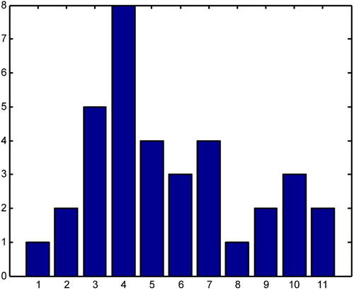
bar(Y) |
Creates a bar chart relative to the vector of frequencies Y. If Y is a matrix it creates multiple bar charts for each row of Y. >> x = [1 2 5 8 4 3 4 1 2 3 2]; >> bar (x)
|
|
bar(x,Y) |
Creates a bar chart relative to the vector of frequencies Y where x is a vector that defines the location of the bars on the x-axis. >> x = - 2.9:0.2:2.9; >> bar (x, exp(-x.*x))
|
|
bar(…,width) |
Creates a bar chart where the bars are given the specified width. By default, the width is 0.8. A width of 1 causes the bars to touch. |
|
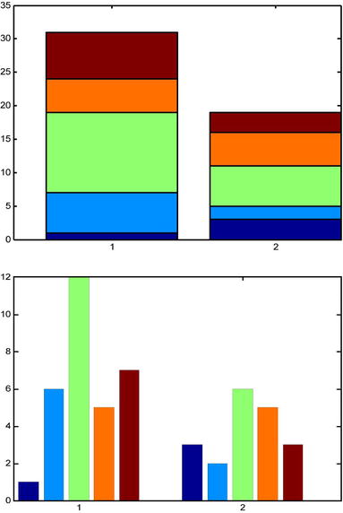
bar(…, ‘style') |
Creates a bar chart with the given style of bars. The possible styles are ‘group’ (the default vertical bar style) and ‘stack’ (stacked horizontal bars). If the matrix is m× n, the bars are grouped in m groups of n bars. >> A = [1 6 12 5 7; 3 2 6 5 3]; >> bar (A, 'stack') >> bar (A, 'group')
|
|
bar(…, color) |
Creates a bar chart where the bars are all of the specified colors (r = red, g = green, b = blue, c = cyan, m = magenta, y = yellow, k = black and w = white). |
|
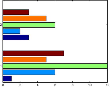
barh(…) |
Creates a horizontal bar chart. >> barh(A,'group')
|
|
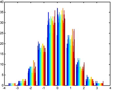
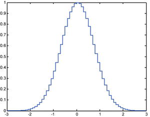
hist(Y) |
Creates a histogram relative to the vector of frequencies Y using 10 equally spaced rectangles. If Y is a matrix, a histogram is created for each of its columns. >> Y = randn(100); >> hist(Y)
|
|
hist(Y,x) |
Creates a histogram relative to the vector of frequencies Y where the number of bins is given by the number of elements in the vector x and the data is sorted according to vector x (if the entries of x are evenly spaced then these are used as the centers of the bins, otherwise the midpoints of successive values are used as the bin edges). |
|
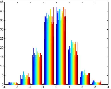
hist(Y,k) |
Creates a histogram relative to the vector of frequencies Y using as many bins as indicated by the scalar k. >> hist(Y, 8)
|
|
[n,x] = hist(…) |
Returns the vectors n and x with the frequencies assigned to each bin of the histogram and the locations of the centers of each bin. |
|
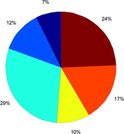
pie(X) |
Creates a pie chart relative to the vector of frequencies X. >> X = [3 5 12 4 7 10]; >> pie(X)
|
|
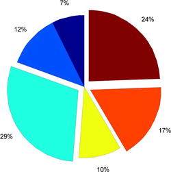
pie(X,Y) |
Creates a pie chart relative to the vector of frequencies X by moving out the sectors for which Yi π 0. >> pie(X,[0 0 1 0 1 1])
|
|
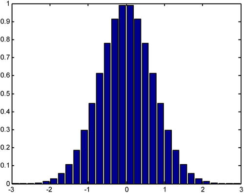
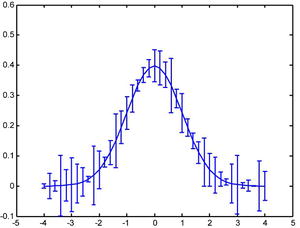
errorbar(x,y,e) |
Plots the function y against x showing the error ranges specified by the vector e. To indicate the confidence intervals, a vertical line of length 2ei is drawn passing through each point (xi , yi) with center (xi , yi). >> x = - 4:.2:4; y = (1/sqrt(2*pi))*exp(-(x.^2)/2); e = rand(size(x))/10; errorbar(x,y,e)
|
|
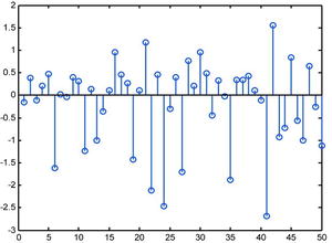
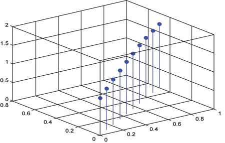
stem (Y) |
Plots the data sequence Y as stems extending from the x-axis baseline to the points indicated by a small circle. >> y = randn (50.1); stem (y)
|
|
stem(X,Y) |
Plots the data sequence Y as a stem diagram with x-axis values determined by X. |
|
stairs (Y) |
Draws a stair step graph of the data sequence Y. |
|
stairs(X,Y) |
Plots a stair step graph of the data Y where the x-values are determined by the vector X. >> x = -3:0.1:3; stairs(x,exp(-x.^2))
|
|
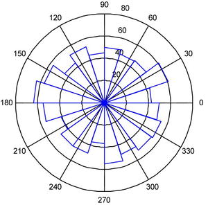
rose (Y) |
Creates an angle histogram showing the distribution of the data Y in 20 angle bins. The angles are given in radians. The radii reflect the number of elements falling into the corresponding bin. >> y = randn(1000,1) * pi; rose(y)
|
|
rose(Y,n) |
Plots an angle histogram of the data Y with n equally spaced bins. The default value of n is 20. |
|
rose(Y,X) |
Plots an angle histogram of the data Y where X specifies the number and location (central angle) of the bins. |
|
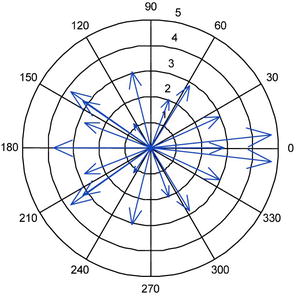
compass (Z) |
Plots a compass diagram of the data Z. For each entry of the vector of complex numbers Z an arrow is drawn with base at the origin and head at the point determined by the entry. >> z = eig(randn(20,20)); compass(z)
|
|
compass(X,Y) |
Equivalent to compass(X+i*Y). |
|
compass (Z, S) or compass (X, Y , S) |
Plots a compass diagram with arrow styles specified by S. |
|
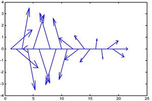
feather(Z) or feather(X,Y) or feather(Z,S) or feather(X,Y,S) |
Produces a plot similar to a compass plot, except the arrows now emanate from equally-spaced points along the x-axis instead of from the origin. >> z = eig(randn(20,20)); feather(z)
|
Curves in Explicit, Implicit, Parametric and Polar Coordinates
The most important MATLAB commands for plotting curves in two dimensions in explicit, polar and implied coordinates are presented in the following table.
|
plot(X,Y) |
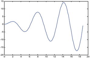
Plots the set of points (X, Y), where X and Y are row vectors. For graphing a function y = f (x) it is necessary to specify a set of points (X, f (X)), where X is the range of variation of the variable x. X and Y can be arrays of the same size, in which case a graph is made by plotting the corresponding points (Xi,Yi) on the same axis. For complex values of X and Y the imaginary parts are ignored. For x = x(t) and y = y(t) with the given parameter t, the specified planar parametric curve graphic variation. >> x = 0:0.1:6*pi; y = x.*sin(x); plot(x,y)
|
|
plot (Y) |
Creates a line plot of the vector Y against its indices. This is useful for plotting time series. If Y is a matrix, plot(Y) creates a graph for each column of Y, presenting them all on the same axes. If the components of the vector are complex, plot(Y) is equivalent to plot(real(Y),imag(Y)). >> Y = [1,3,9,27,81,243,729]; plot(Y)
|
|
plot (X, Y, S) |
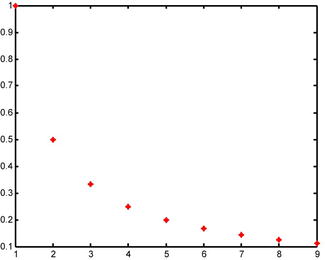
Creates a plot of Y against X as described by plot(X,Y) with the settings defined in S. Usually S consists of two characters between single quotes, the first sets the color of the line graph and the second specifies the marker or line type. The possible values of colors and characters are, respectively, as follows: y (yellow), m (magenta), c (cyan), r (red), g (green), b (blue), w (white), k (black), . (point), o (circle), x (cross), s (square), d (diamond), ^ (upward pointing triangle), v (downward pointing triangle), > (right pointing triangle), < (left pointing triangle), p (pentagram), h (hexagram), + (plus sign), * (asterisk), - (solid line), -- (dashed line),: (dotted line), -. (dash-dot line). >> plot([1,2,3,4,5,6,7,8,9],[1, 1/2, 1/3,1/4,1/5,1/6, 1/7,1/8,1/9],'r *')
|
|
plot (X1,Y1,S1,X2,Y2,S2,…) |
Combines the plots for the triples (Xi, Yi, Si). This is a useful way of representing various functions on the same graph. |
|
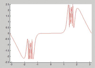
fplot (‘f’, [xmin, xmax]) |
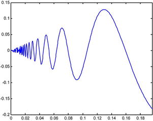
Graphs the explicit function y = f (x) in the specified range of variation for x. >> fplot('x*sin(1/x)', [0,pi/16])
|
|
fplot(‘f’,[xmin, xmax, ymin, ymax], S) |
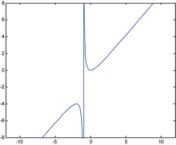
Graphs the explicit function y = f (x) in the specified intervals of variation for x and y, with options for color and characters given by S. >> fplot('x^2/(x+1)', [-12,12,-8, 8])
|
|
fplot(‘f’,[xmin,xmax],…,t) |
Graphs the function f with relative error tolerance t. |
|
fplot(‘f’,[xmin, xmax],…,n) |
Graphs the function f with a minimum of n + 1 points where the maximum step size is (xmax-xmin)/n. |
|
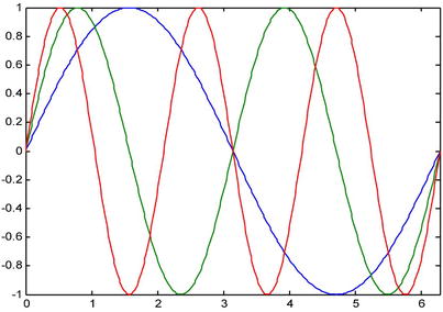
fplot(‘[f1,f2,…,fn]’, [xmin, xmax, ymin, ymax], S) |
Graphs the functions f1, f2,…, fn on the same axes in the specified ranges of variation of x and y and with the color and markers given by S. >> fplot('[sin(x), sin(2*x), sin(3*x)]', [0,2*pi])
>> fplot('[sin (x), sin(2*x), sin(3*x)]', [0, 2 * pi],'k *')
|
|
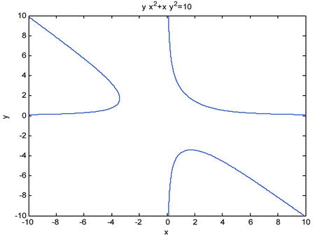
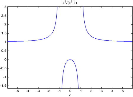
ezplot (‘f’, [xmin xmax]) |
Graphs the explicit function y = f (x) or implicit function f(x,y) = k in the given range of variation of x. The range of variation of the variable can be omitted. >> ezplot('y*x^2+x*y^2=10',[-10,10])
>> ezplot('x ^ 2-/(x^2-1)')
|
|
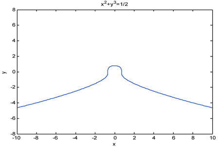
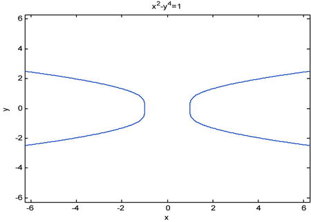
ezplot (‘f’, [xmin, xmax, ymin, ymax]) |
Graphs the explicit function y = f (x) or the implicit function f(x,y) = k for the given intervals of variation of x and y (which can be omitted). >> ezplot('x^2+y^3=1/2',[-10,10,-8,8])
>> ezplot('x^2-y^4=1')
|
|
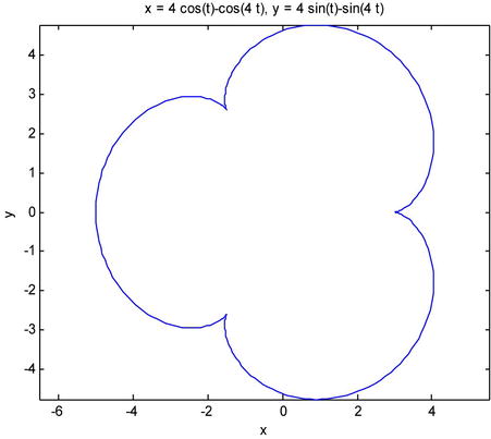
ezplot(x,y) |
Graphs the planar parametric curve x = x (t) and y = y(t) for 0 ≤ t < 2π. >> ezplot('4 * cos(t) - cos(4*t)', ' 4 * sin(t) - sin(4*t)')
|
|
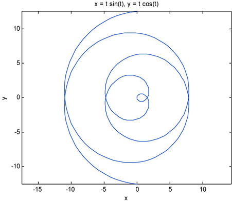
ezplot (‘f’, [xmin xmax]) |
Graphs the planar parametric curve x = x (t) and y = y(t) for xmin < t < xmax. >> ezplot('t*sin(t)', 't*cos(t)',[-4*pi,4*pi]
|
|
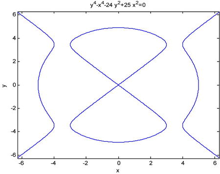
ezplot (‘f’) |
Graphs the curve f where the coordinates range over the default domain [-2π, 2π]. >> ezplot('y^4-x^4-24*y^2+25*x^2=0')
|
|
loglog(X,Y) |
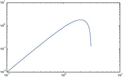
Produces a plot similar to plot(X,Y), but with a logarithmic scale on the two axes. >> x=0:0.1:pi; y=x.*sin(x); loglog(x,y)
|
|
semilogx(X,Y) |
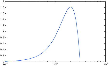
Produces a plot similar to plot(X,Y), but with a logarithmic scale on the x-axis and a normal scale on the y-axis. >> x=0:0.1:pi; y=x.*sin(x); semilogx(x,y)
|
|
semilogy(X,Y) |
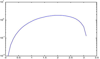
Produces a plot similar to plot(X,Y), but with a logarithmic scale on the y-axis and a normal scale on the x-axis. >> x=0:0.1:pi; y=x.*sin(x); semilogy(x,y)
|
|
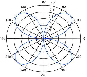
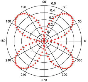
polar (α, r) |
Draws the curve >> t=0:0.1:2*pi;r=sin(t).*cos(t); polar(t,r)
|
|
polar (α, r, S) |
Draws the curve >> t=0:0.05:2*pi;r=sin(t).*cos(t); polar(t,r,'*r')
|
|
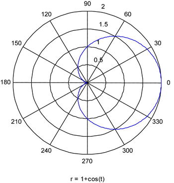
ezpolar (r) ezpolar (r, [a, b]) |
Draws the curve >> ezpolar ('1 + cos (t)')
|
|
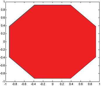
fill (X, Y, C) |
Draws the filled polygon whose vertices are given by the components (Xi , Yi) of the specified vectors X and Y. The vector C, which is of the same size as X and Y, specifies the colors assigned to the corresponding points. The Ci values may be: ‘r’, ‘g’, ‘b’, ‘c’, ‘m’, ‘y’, ‘w’, ‘k’, whose meanings we already know. If C is a single character, all vertices of the polygon will be assigned the specified color. If X and Y are matrices of the same size then several polygons will be created, each corresponding to the columns of the matrices. In this case, C can be a row vector specifying the color of each polygon, or it can be a matrix specifying the color of the vertices of the polygons. >> t = (1/16:1 / 8:1)'* 2 * pi; x = sin(t); y = cos(t); fill(x, y, 'r')
|
|
fill(X1,Y1,C1,…) |
Draws the filled polygon with vertex coordinates and colors given by (Xi, Yi, Ci). |


MATLAB includes commands that allow you to plot space curves in three dimensions. The following table presents the most important commands.
|
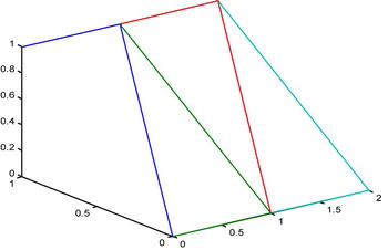
plot3 (X, Y, Z) |
Draws a 3D line plot by joining the sequence of points determined by (X, Y, Z) by lines, where X, Y and Z are row vectors. X, Y and Z can also be parametric coordinates or matrices of the same size, in which case a graph is made for each triplet of rows, on the same axes. For complex values of X, Y and Z, the imaginary parts are ignored. >> X = [0 1 1 2; 1 1 2 2; 0 0 1 1]; Y = [1 1 1 1; 1 0 1 0; 0 0 0 0]; Z = [1 1 1 1; 1 0 1 0; 0 0 0 0]; >> plot3 (X, Y, Z)
>> t = 0:pi/100:20 * pi; plot3 (2 * sin(2*t), 2 * cos(2*t), 4 * t)
|
|
plot3 (X, Y, Z, S) |
Produces the line plot plotting (X,Y,Z) with the settings defined in S. S usually consists of two characters between single quotes, the first of which sets the color of the line graph and the second determines the line or marker properties. The possible settings have already been described above for the plot command. |
|
plot3(X1,Y1,Z1,S1, X2,Y2,Z2,S2,X3, Y3, Z3, S3,…) |
Combines 3D line plots for the quadruples (Xi, Yi, Zi, Si) on the same axes. This is a useful way of representing various functions on the same graph. |
|
fill3(X,Y,Z,C) |
Draws the filled polygon whose vertices are given by the triples of components (Xi, Yi, Zi) of the column vectors X, Y and Z. C is a vector of the same size as X, Y and Z, which specifies the color Ci at each vertex (Xi, Yi, Zi). The Ci values can be ‘r’, ‘g’, ‘b’, ‘c’, ‘m’, ‘y’, ‘w’, ‘k’, whose meanings we already know. If C is a single character, all vertices will be given this color. If X, Y and Z are matrices of the same size, several polygons corresponding to each triplet column vector (X.j, Y.j, Z.j) will be drawn. In this case, C can be a row vector of elements Cj determining the unique color of each polygon corresponding to (X.j, Y.j, Z.j). C can also be a matrix of the same dimension as X, Y and Z, in which case its elements determine the colors of each vertex (Xijk, Yijk, Zijk) of the set of polygons. >> X = [0 1 1 2; 1 1 2 2; 0 0 1 1]; Y = [1 1 1 1; 1 0 1 0; 0 0 0 0]; Z = [1 1 1 1; 1 0 1 0; 0 0 0 0]; C = [0.5000 1.0000 1.0000 0.5000; 1.0000 0.5000 0.5000 0.1667; 0.3330 0.3330 0.5000 0.5000]; fill3(X,Y,Z,C)
|
|
fill3(X1,Y1,Z1,C1, X2, Y2, Z2, C2,…) |
Draws the filled polygon whose vertices and colors are given by (Xi, Yi, Zi, Ci). |
|
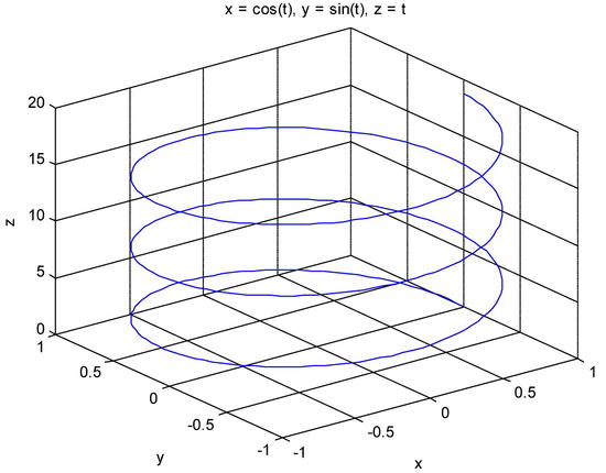
ezplot3(x(t), y(t), z(t)) ezplot3(x(t),y(t),z(t), [tmin,tmax]) |
Draws the space curve defined by the given three parametric components. Draws the space curve defined by the given three parametric components for the specified range of variation of the parameter. >> ezplot3('sin (t)', 'cos (t)', ', [0, 6 * pi])
|
Explicit and Parametric Surfaces: Contour Plots
MATLAB includes commands that allow you to represent surfaces defined by equations of the form z = f(x,y). The first step is to use the command meshgrid, which defines the array of points (X, Y) at which the function will be evaluated. Then the command surf is used to create the surface.
The command mesh is also used to produce a mesh plot that is defined by a function z = f(x,y), so that the points on the surface are represented on a network determined by the z values given by f(x,y) for corresponding points of the plane (x, y). The appearance of a mesh plot is like a fishing net, with surface points forming the nodes of the network.
It is also possible to represent the level curves of a surface by using the command contour. These curves are characterized as being the set of points (x,y) in the plane for which the value f(x,y) is some fixed constant.
The following table lists the MATLAB commands which can be used to produce mesh and contour representations of surfaces both in explicit and parametric form.
|
[X, Y] = meshgrid(x,y) |
Creates a rectangular grid by transforming the monotonically increasing grid vectors x and y into two matrices X and Y specifying the entire grid. Such a grid can be used by the commands surf and mesh to produce surface graphics. |
|
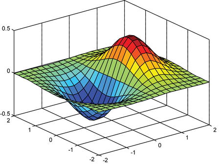
surf(X,Y,Z,C) |
Represents the explicit surface z = f(x,y) or the parametric surface x = x(t,u), y = y(t,u), z = z(t,u), using the colors specified in C. The C argument can be omitted. >> [X, Y] = meshgrid(-2:.2:2,-2:.2:2); Z = X. * exp(-X.^2-Y.^2); surf(X, Y, Z)
|
|
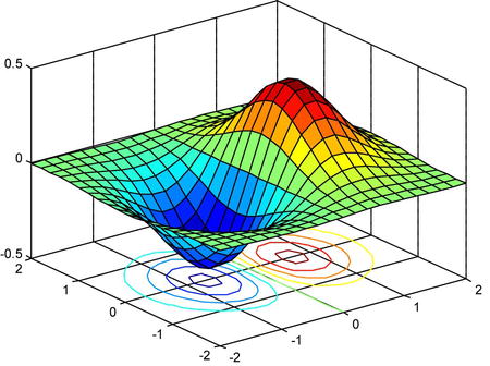
surfc(X,Y,Z,C) |
Represents the explicit surface z = f(x,y) or the parametric surface x = x(t,u), y = y(t,u), z = z(t,u), together with a contour plot of the surface. The contour lines are projected onto the xy-plane. >> [X, Y] = meshgrid(-2:.2:2,-2:.2:2); Z = X. * exp(-X.^2-Y.^2); surfc(X, Y, Z)
|
|
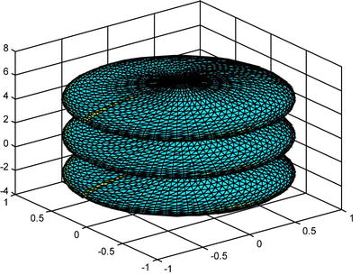
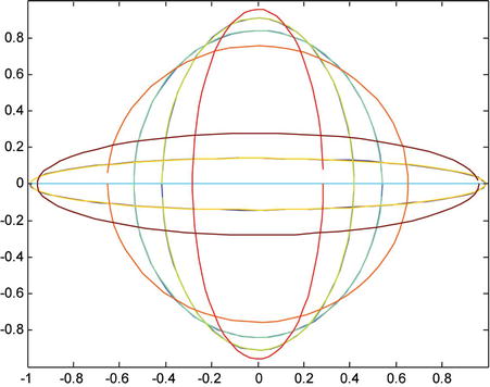
surfl (X, Y, Z) |
Represents the explicit surface z = f(x,y) or the parametric surface x = x(t,u), y = y(t,u), z = z(t,u), with colormap-based lighting. >> r =(0:0.1:2*pi)'; t =(-pi:0.1:2*pi); X = cos(r) * sin(t); Y = sin(r) * sin(t); Z = ones(size(r),1)'* t; surfl(X, Y, Z)
|
|
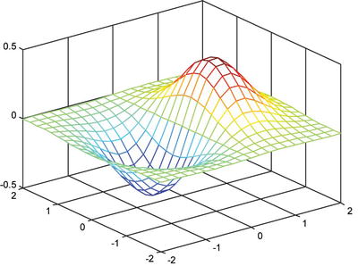
mesh(X,Y,Z,C) |
Represents the explicit surface z = f(x,y) or the parametric surface x = x(t,u), y = y(t,u), z = z(t,u), drawing the grid lines that compose the mesh with the colors specified by C (optional). >> [X, Y] = meshgrid(-2:.2:2,-2:.2:2); Z = X. * exp(-X.^2-Y.^2); mesh(X, Y, Z)
|
|
meshz(X,Y,Z,C) |
Represents the explicit surface z = f(x,y) or the parametric surface x = x(t,u), y = y(t,u), z = z(t,u) adding a ‘curtain’ around the mesh. |
|
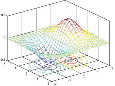
meshc(X,Y,Z,C) |
Represents the explicit surface z = f(x,y) or the parametric surface x = x(t,u), y = y(t,u), z = z(t,u) together with a contour plot of the surface. The contour lines are projected on the xy-plane. >> [X, Y] = meshgrid(-2:.2:2,-2:.2:2); Z = X. * exp(-X.^2-Y.^2); meshc(X, Y, Z)
|
|
contour (Z) |
Draws a contour plot of the matrix Z, where Z is interpreted as heights of the surface over the xy-plane. The number of contour lines is selected automatically. >> [X, Y] = meshgrid(-2:.2:2,-2:.2:2); Z = X. * exp(-X.^2-Y.^2); >> contour(Z)
|
|
contour(Z,n) |
Draws a contour plot of the matrix Z using n contour lines. >> [X, Y] = meshgrid(-2:.2:2,-2:.2:2); Z = X. * exp(-X.^2-Y.^2); >> contour(Z)
|
|
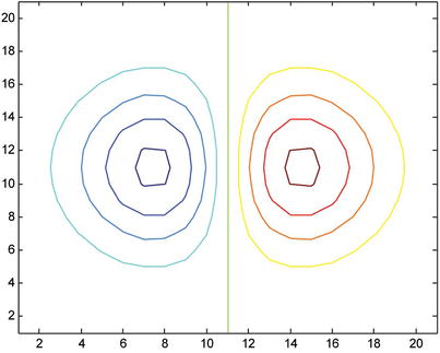
contour (x, y, Z, n) |
Draws a contour plot of the matrix Z with n contour lines and using the x-axis and y-axis values specified by the vectors x and y. >> r =(0:0.1:2*pi); t =(-pi:0.1:2*pi); X = cos(r) * cos(t);Y = sin(r) * sin(t);Z = ones(size(r),1)'* t; >> contour(X, Y, Z)
|
|
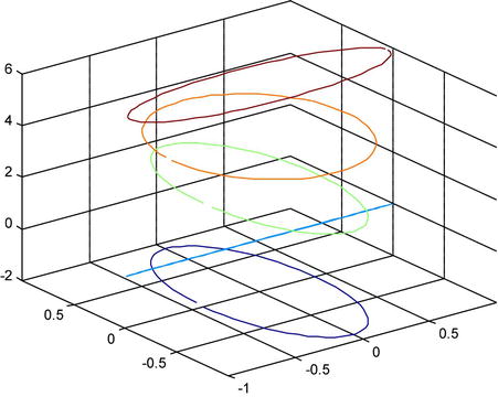
contour3 (Z), contour3 (Z, n) y contour3 (x, y, Z, n) |
Draws three-dimensional contour plots. >> r =(0:0.1:2*pi); t =(-pi:0.1:2*pi); X = cos (r) * cos(t);Y = sin(r) * sin(t);Z = ones(size(r),1)'* t; >> contour3(X, Y, Z)
|
|
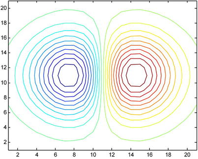
contourf (…) |
Draws a contour plot and fills in the areas between the isolines. >> r =(0:0.1:2*pi); t =(-pi:0.1:2*pi); X = cos(r) * cos(t);Y = sin(r) * sin(t);Z = ones(size(r),1)'* t; >> contourf(X, Y, Z)
|
|
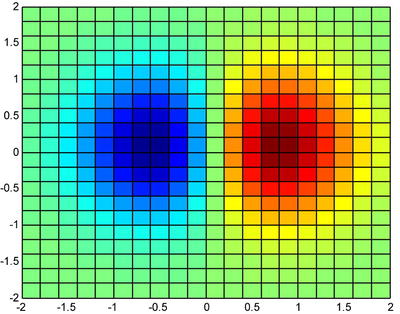
pcolor (X, Y, Z) |
Draws a ‘pseudocolor’ contour plot determined by the matrix (X, Y, Z) using a color representation based on densities. This is often called a density plot. >> [X, Y] = meshgrid(-2:.2:2,-2:.2:2); Z = X. * exp(-X.^2-Y.^2); meshc(X, Y, Z) >> pcolor(X, Y, Z)
|
|
trimesh(Tri, X, Y, Z, C) |
Creates a triangular mesh plot. Each row of the matrix Tri defines a simple triangular face and C defines colors as in surf. The C argument is optional. |
|
trisurf(Tri,X,Y,Z,C) |
Creates a triangular surface plot. Each row of the matrix Tri defines a simple triangular face and C defines colors as in surf. The C argument is optional. |
Three-Dimensional Geometric Forms
The representation of cylinders, spheres, bars, sections, stems, waterfall charts and other three-dimensional geometric objects is possible with MATLAB. The following table summarizes the commands that can be used for this purpose.

Specialized Graphics
MATLAB provides commands to create various plots and charts (filled areas, comet, contour, mesh, surface and scatter plots, Pareto charts, and stair step graphs). You can also modify axes specifications, and there is an easy to use function plotter. The following table presents the syntax of these commands.
|
area(Y) area(X, Y) area(…,ymin) |
Creates an area graph displaying the elements of the vector Y as one or more curves, filling the area beneath the curve. Identical to plot(X,Y), except the area between 0 and Y is filled. Specifies the base value for the fill area (default 0) . >> Y = [1, 5, 3; 3, 2, 7; 1, 5, 3; 2, 6, 1]; area(Y)
|
|
box on, box off |
Displays/does not display the boundary of the current axes. |
|
comet(y) comet(x, y) |
Creates an animated comet graph of the vector y. Plots the comet graph of the vector y versus the vector x. >> t = - pi:pi/200:pi;comet(t,tan(sin(t))-sin(tan(t)))
|
|
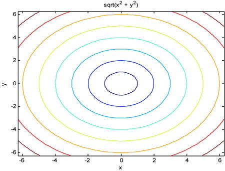
ezcontour(f) ezcontour(f, domain) ezcontour(…,n) |
Creates a contour plot of f(x,y) in the domain [-2π, 2π] × [-2p, 2π]. Creates a contour plot of f(x,y) in the given domain. Creates a contour plot of f(x,y) over an n×n grid. >> ezcontour('sqrt(x^2 + y^2)')
|
|
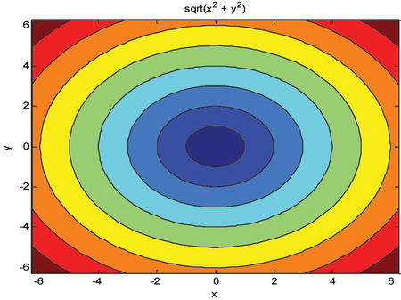
ezcontourf (f) ezcontourf (f, domain) ezcontourf(…,n) |
Creates a filled contour plot of f(x,y) in the domain [-2π, 2π] × [-2p, 2π]. Creates a filled contour plot of f(x,y) in the given domain. Creates a filled contour plot of f(x,y) over an n×n grid. >> ezcontourf('sqrt(x^2 + y^2)')
|
|
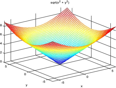
ezmesh(f) ezmesh(f,domain) ezmesh(…,n) ezmesh (x, y, z) ezmesh (x, y, z, domain) ezmesh(…, ‘circ’) |
Creates a mesh plot of f(x,y) over the domain [-2p, 2π] × [-2π, 2π]. Creates a mesh plot of f(x,y) over the given domain. Creates a mesh plot of f(x,y) using an n×n grid. Creates a mesh plot of the parametric surface x = x(t,u), y = y(t,u), z = z(t,u), t,uŒ[-2π, 2π]. Creates a mesh plot of the parametric surface x = x(t,u), y = y(t,u), z = z(t,u), t,uŒ domain. Creates a mesh plot over a disc centered on the domain. >> ezmesh ('sqrt(x^2 + y^2)')
|
|
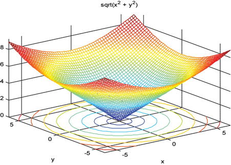
ezmeshc (f) ezmeshc (f, domain) ezmeshc(…,n) ezmeshc (x, y, z) ezmeshc (x, y, z, domain) ezmeshc(…, ‘circ’) |
Creates a combination of mesh and contour graphs. >> ezmeshc ('sqrt(x^2 + y^2)')
|
|
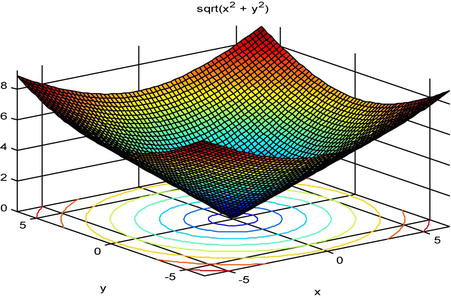
ezsurf (f) ezsurf (f, domain) ezsurf(…,n) ezsurf (x, y, z) ezsurf (x, y, z, domain) ezsurf(…, ‘circ’) |
Creates a colored surface plot. >> ezsurf('sqrt(x^2 + y^2)')
|
|
ezsurfc (f) ezsurfc (f, domain) ezsurfc(…,n) ezsurfc (x, y, z) ezsurfc (x, y, z, domain) ezsurfc(…, ‘circ’) |
Creates a combination of surface and contour plots. >> ezsurfc('sqrt(x^2 + y^2)')
|
|
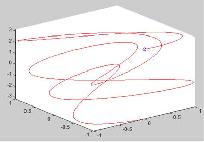
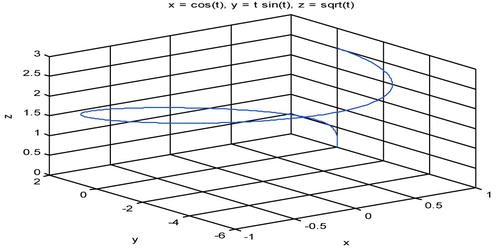
ezplot3 (x, y, z) ezplot3 (x, y, z, domain) ezplot3(…, ‘animate’) |
Plots the 3D parametric curve x = x (t), y(t) = y, z(t) = z tŒ[-2π, 2p]. Plots the 3D parametric curve x = x (t), y(t) = y, z(t) = z tŒdomain. Creates a 3D animation of a parametric curve. >> ezplot3('cos(t)','t.*sin(t)','sqrt(t)')
|
|
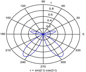
ezpolar(f) ezpolar(f, [a, b]) |
Graphs the polar curve r = f (c) with cŒ[0, 2π]. Graphs the polar curve r = f (c) with cŒ[a, b]. ezpolar ('sin(2*t). * cos(3*t)', [0 pi])
|
|
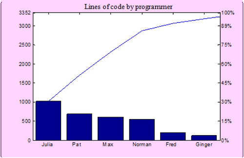
pareto(Y) pareto(X,Y) |
Creates a Pareto chart relative to the vector of frequencies Y. Creates a Pareto chart relative to the vector of frequencies Y whose elements are given by the vector X. >> lines_of_code = [200 120 555 608 1024 101 57 687]; coders =… {'Fred', 'Ginger', 'Norman', 'Max', 'Julie', 'Wally', 'Heidi', 'Pat'}; Pareto (lines_of_code, coders) title ('lines of code by programmer')
|
|
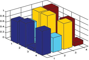
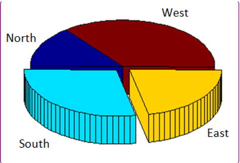
pie.3 (X) pie.3(X, explode) |
Creates a 3D pie chart for frequencies X. Creates a detached 3D pie chart. >> ft3 ([2 4 3 5], [0 1 1 0], {'North', 'South', 'East', 'West'})
|
|
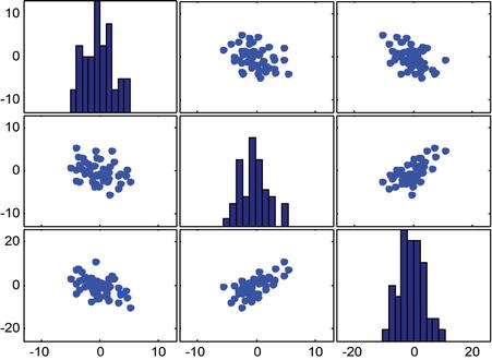
plotmatrix(X, Y) |
Creates a scatter plot of the columns of X against the columns of Y. >> x = randn (50,3); y = x * [- 1 2 1; 2 0 1; 1-2-3;]';plotmatrix (y)
|
|
stairs (Y) stairs(X, Y) stairs(…,linespec) |
Draws a stair step graph of the elements of Y. Draws a stair step graph of the elements of Y at the locations specified by X. In addition, specifies line style, marker symbol and color. >> x = linspace(-2*pi,2*pi,40);stairs(x,sin(x))
|
|
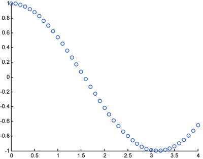
scatter(X,Y,S,C) scatter(X,Y) scatter(X,Y,S) scatter(…, marker) scatter(…, ‘filled’) |
Creates a scatter plot, displaying circles at the locations specified by X and Y. S specifies the circle size and C the color. The circles can be filled and different markers can be specified. |
|
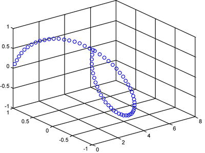
scatter3(X,Y,Z,S,C) scatter3(X,Y,Z) scatter3(X,Y,Z,S) scatter3(…,marker) scatter(…,‘filled’) |
Creates a 3D scatter plot determined by the vectors X, Y, Z. Colors and markers can be specified. >> x=(0:0.1:4); >> scatter(x,cos(x))
>> x=(0:0.1:2*pi); >> scatter3 (x, cos(x), sin(x))
|


MATLAB includes many different commands which enable graphics handling, including titles, legends and axis labels, addition of text to plots, and adjustment of coloring and shading. The most important commands are summarized in the following table.
|
title (‘text’) |
Adds a title to the top of the current axes. |
|
xlabel (‘text’) |
Adds an x-axis label. |
|
ylabel (‘text’) |
Adds a y-axis label. |
|
zlabel (‘text’) |
Adds a z-axis label. |
|
clabel(C,h) |
Labels contour lines of a contour plot with a ‘+’, rotating the labels so they are positioned on the inside of the contour lines. |
|
clabel(C,h,v) |
Labels contour lines of a contour plot only for the levels given by the vector v, rotating the labels so they are positioned on the inside of the contour lines. |
|
datetick (axis) |
Creates date formatted tick labels for the specified axis (‘x’, ‘y’ or ‘z’). |
|
datetick (axis, date) |
Creates date formatted tick labels for the specified axis (‘x’, ‘y’ or ‘z’) with the given date format (an integer between 1 and 28). |
|
legend (‘string1’, ‘string2’,…) |
Displays a legend in the current axes using the specified strings to label each set of data. |
|
legend(h,‘string1’, ‘string2’,…) |
Displays a legend on the plot containing the objects identified by the vector h and uses the specified strings to label the corresponding graphics objects. |
|
legend (‘off’), |
Deletes the current axes legend. |
|
text (x, y, ‘text’) |
Places the given text at the point (x, y) within a 2D plot. |
|
text (x, y, z, ‘text’) |
Places the given text at the point (x, y, z) in a 3D plot. |
|
gtext (‘text’) |
Allows you to place text at a mouse-selected point in a 2D plot. |
|
grid |
Adds grid lines to 2D and 3D plots. Grid on adds major grid lines to the axes, grid off removes all grid lines from the current axes. The command grid toggles the visibility of the major grid lines. |
|
hold |
Controls whether the current graph is cleared when you make subsequent calls to plotting functions (the default), or adds a new graph to the current graph, maintaining the existing graph with all its properties. The command hold on retains the current graph and adds another graph to it. The command hold off resets to default properties before drawing a new graph. |
|
axis ([xmin xmax ymin ymax zmin zmax]) |
Sets the axes limits. |
|
axis (‘auto’) |
Computes the axes limits automatically (xmin = min (x), xmax = max(x)). |
|
axis (axis) |
Freezes the scaling at the current limits, so that if hold is on, subsequent plots use the same limits. |
|
V = axis |
Returns a row vector V containing scaling factors for the x-, y-, and z-axes. V has four or six components depending on whether the plot is 2D or 3D, respectively. |
|
axis (‘xy’) |
Uses Cartesian coordinates with the origin at the bottom left of the graph. |
|
axis (‘tight’) |
Sets the axis limits to the range of the data. |
|
axis (‘ij’) |
Places the origin at the top left of the graph. |
|
axis (‘square’) |
Makes the current axes region a square (or a cube when three-dimensional). |
|
axis (‘equal’) |
Uses the same scaling factor for both axes. |
|
axis (‘normal’) |
Removes the square and equal options. |
|
axis (‘off’) |
Turns off all axis lines, tick marks, and labels, keeping the title of the graph and any text. |
|
axis (‘on’) |
Turns on all axis lines, tick marks, and labels. |
|
subplot (m, n, p) |
Divides the current figure into an m×n grid and creates axes in the grid position specified by p. The grids are numbered by row, so that the first grid is the first column of the first row, the second grid is the second column of the first row, and so on. |
|
plotyy(X1,Y1,X2,Y2) plotyy(X1,Y1,X2,Y2,) ‘function’) plotyy(X1,Y1,X2,Y2, ‘function1’, ‘function2’) |
Plots X1 versus Y1 with y-axis labeling on the left and plots X2 versus Y2 with y-axis labeling on the right. Same as the previous command, but using the specified plotting function (plot, loglog, semilogx, semilogy, stem or any acceptable function h = function(x,y)) to plot the graph. Uses function1(X1,Y1) to plot the data for the left axis and function2(X2,Y2) to plot the data for the right axis. |
|
axis ([xmin xmax ymin ymax zmin zmax]) |
Sets the x-, y-, and z-axis limits. Also accepts the options ‘ij’, ‘square’, ‘equal’, etc., identical to the equivalent two-dimensional command. |
|
view ([x, y, z]) |
Sets the viewing direction to the Cartesian coordinates x, y, and z. |
|
view([as, el]) |
Sets the viewing angle for a three-dimensional plot. The azimuth, az, is the horizontal rotation about the z-axis as measured in degrees from the negative y-axis. Positive values indicate counterclockwise rotation of the viewpoint. el is the vertical elevation of the viewpoint in degrees. Positive values of elevation correspond to moving above the object; negative values correspond to moving below the object. |
|
hidden |
Hidden line removal draws only those lines that are not obscured by other objects in a 3-D view. The command hidden on hides such obscured lines while hidden off shows them. |
|
shading |
Controls the type of shading of a surface created with the commands surf, mesh, pcolor, fill and fill3. The option shading flat gives a smooth shading, shading interp gives a dense shadow and shading faceted (default) yields a standard shading. |
|
colormap (M) |
Sets the colormap to the matrix. M must have three columns and only contain values between 0 and 1. It can also be a matrix whose rows are vectors of RGB type [r g b]. There are some pre-defined arrays M, which are as follows: jet (p), HSV (p), hot (p), cool (p), spring (p), summer (p), autumn (p), winter (p), gray (p), bone (p), copper (p), pink (p), lines (p). All arrays have 3 columns and p rows. For example, the syntax colormap (hot (8)) sets hot (8) as the current colormap. |
|
brighten (p) |
Adjusts the brightness of the figure. If 0 < p < 1, the figure will be brighter, and if -1<p<0 the figure will be darker. |
|
image (A) |
Creates an image graphics object by interpreting each element in a matrix as an index into the figure’s colormap or directly as RGB values, depending on the data specified. |
|
pcolor (A) |
Produces a pseudocolor plot, i.e. a rectangular array of cells with colors determined by A. The elements of A are linearly mapped to an index into the current colormap. |
|
caxis ([cmin cmax]) |
Sets the color limits to the specified minimum and maximum values. Data values less than cmin or greater than cmax map to cmin and cmax, respectively. Values between cmin and cmax linearly map to the current colormap. |
|
h = figure figure(h) |
Creates a figure graphics object with name h. Makes the figure identified by h the current figure, makes it visible, and attempts to raise it above all other figures on the screen. The current figure is the target for graphics output. The command close(h) deletes the figure identified by h. The command whitebg(h) complements all the colors of the figure h. The clf command closes the current figure. The command graymon sets defaults for graphics properties to produce more legible displays for grayscale monitors. The refresh command redraws the figure. |
|
e = axes axes(e) |
Creates axes objects named e. Makes the existing axes e the current axes and brings the figure containing it into focus. The command gca returns the name of the current axes. The command cla deletes all objects related to the current axes. |
|
l = line(x,y) or l = line (x, y, z) |
Creates, as an object of name l, the line joining the points X, Y in the plane or the points X, Y, Z in space. |
|
p = (X, Y, C) patch or patch(X,Y,Z,C) |
Creates an opaque polygonal area p that is defined by the set of points (X, Y) in the plane or (X, Y, Z) in space, and whose color is given by C. |
|
s = surface(X,Y,Z,C) |
Creates the parametric surface s defined by X, Y and Z and whose color is given by C. |
|
i = image (C) |
Creates an image i from the matrix C. Each element of C specifies the color of a rectangular segment in the image. |
|
t = text (x, y, ‘string’) or t = text (x, y, z, ‘string’) |
Creates the text t defined by the chain, located at the point (x, y) in the plane, or at the point (x, y, z) in space. |
|
set (h, ‘property1’, ‘property2’,…) |
Sets the named properties for the object h (gca for limits of axes), gcf, gco, gcbo, gcbd, colors, etc. |
|
get (h, ‘property’) |
Returns the current value of the given property of the object h. |
|
object = gco |
Returns the name of the current object. |
|
rotate(h, v, α,[p, q, r]) |
Rotates the object h by an angle α about an axis of rotation described by the vector v from the point (p, q, r). |
|
reset (h) |
Updates all properties assigned to the object h replacing them with their default values. |
|
delete (h) |
Deletes the object h. |
In addition, the most typical properties of graphics objects in MATLAB are the following:
|
Object |
Properties |
Possible values |
|---|---|---|
|
Figure |
Color (background color) |
‘y’, ‘m’, ‘c’, ‘r’, ‘g’, ‘b’, ‘w’, ‘k’ |
|
ColorMap (map color) |
hot(p), gray(p), pink(p),.... | |
|
Position (figure position) |
[left, bottom, width, height] | |
|
Name (figure name) |
string name | |
|
MinColorMap (min. color no.) |
minimum number of colors for map | |
|
NextPlot (graph. mode following.) |
new, add, replace | |
|
NumberTitle (no. in the figure title) |
on, off | |
|
Units (units of measurement) |
pixels, inches, centimeters, points | |
|
Resize (size figure with mouse) |
on (can be changed), off (cannot be changed) | |
|
Axes |
Box (box axes) |
on, off |
|
Color (color of the axes) |
‘y’, ‘c’, ‘r’, ‘g’, ‘b’, ‘w’, ‘k’ | |
|
P:System.Windows.Forms.DataGrid.GridLineStyle (line for mesh) |
‘-’, ‘--’, ‘:’, ‘-.’ | |
|
Position (origin position) |
[left, bottom, width, height] | |
|
TickLength (distance between marks) |
a numeric value | |
|
TickDir (direction of marks) |
in, out | |
|
Units (units of measurement) |
pixels, inches, centimeters, points | |
|
View (view) |
[azimuth, elevation] | |
|
FontAngle (angle of source) |
normal, italic, oblique | |
|
FontName (name of source) |
the name of the source text | |
|
FontSize (font size) |
numeric value | |
|
T:System.Windows.FontWeight (weight) |
light, normal, demi, bold | |
|
DrawMode property (drawing mode) |
normal, fast | |
|
Xcolor, Ycolor, Zcolor (axes color) |
[min, max] | |
|
XDir, Jdir, ZDir (axes direction) |
normal (increasing from left to right), reverse | |
|
XGrid, YGrid, Zgrid (grids) |
on, off | |
|
XLabel, YLabel, Zlabel (tags) |
string containing the text of labels | |
|
XLim, YLim, ZLim (limit values) |
[min, max] (range of variation) | |
|
XScale, YScale, ZScale (scales) |
linear, log (log) | |
|
XTick,YTick,ZTick (marks) |
[m1,m2,…] (position of marks on axis) | |
|
Line |
Color (color of the line) |
‘y’, ‘m’, ‘c’, ‘r’, ‘g’, ‘b’, ‘w’, ‘k’ |
|
LineStyle (line style) |
‘-’, ‘--’, ‘:’, ‘-.’, ‘+’, ‘*’, ‘.’, ‘x’ | |
|
LineWidth (line width) |
numeric value | |
|
Visible (visible line or not displayed.) |
on, off | |
|
Xdata, Ydata, Zdata (coordinates.) |
set of coordinates of the line | |
|
Text |
Color (text color) |
‘y’, ‘m’, ‘c’, ‘r’, ‘g’, ‘b’, ‘w’, ‘k’ |
|
FontAngle (angle of source) |
normal, italic, oblique | |
|
FontName (name of source) |
the name of the source text | |
|
FontSize (font size) |
numeric value | |
|
T:System.Windows.FontWeight (weight) |
light, normal, demi, bold | |
|
HorizontalAlignment (hor. setting.) |
left, center, right | |
|
VerticalAlignment (adjust to vert.) |
top, cap, middle, baseline, bottom | |
|
Position (position on screen) |
[x, y, z] (text coordinates) | |
|
Rotation (orientation of the text) |
0, ±90, ±180, ±270 | |
|
Units (units of measurement) |
pixels, inches, centimeters, points | |
|
String (text string) |
the text string | |
|
Surface |
CDATA (color of each point) |
color matrix |
|
Edgecolor (color grids) |
‘y’,‘m’,…, none, flat, interp | |
|
Facecolor (color of the faces) |
‘y’,‘m’,…, none, flat, interp | |
|
LineStyle (line style) |
‘-’, ‘--’, ‘:’, ‘-.’, ‘+’, ‘*’, ‘.’, ‘x’ | |
|
LineWidth (line width) |
numeric value | |
|
MeshStyle (lines in rows and col.) |
row, Columbia, both | |
|
Visible (visible line or not displayed.) |
on, off | |
|
Xdata, Ydata, Zdata (coordinates) |
set of coordinates of the surface | |
|
Patch |
CDATA (color of each point) |
color matrix |
|
Edgecolor (color of the axes) |
‘y’,‘m’,…, none, flat, interp | |
|
Facecolor (color of the faces) |
‘y’,‘m’,…, none, flat, interp | |
|
LineWidth (line width) |
numeric value | |
|
Visible (visible line or not displayed.) |
on, off | |
|
Xdata, Ydata, Zdata (coordinates) |
set of coordinates of the surface | |
|
Image |
CDATA (color of each point) |
color matrix |
|
Xdata, Ydata (coordinates) |
set of coordinates of the image |
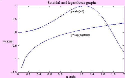
Here are some illustrative examples.
>> x=linspace(0,2,30);
y=sin(x.^2);
plot(x,y)
text(1,0.8, 'y=sin(x^2)')
hold on
z=log(sqrt(x));
plot(x,z)
text(1,-0.1, 'y=log(sqrt(x))')
xlabel('x-axis'),
ylabel('y-axis'),
title(Sinoidal and logarithmic graphs'),
>> subplot(2,2,1);
ezplot('sin(x)',[-2*pi 2*pi])
subplot(2,2,2);
ezplot('cos(x)',[-2*pi 2*pi])
subplot(2,2,3);
ezplot('csc(x)',[-2*pi 2*pi])
subplot(2,2,4);
ezplot('sec(x)',[-2*pi 2*pi])

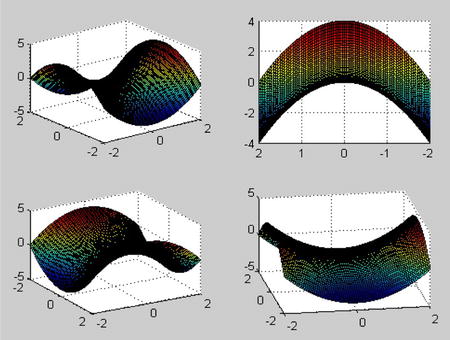
>> [X,Y] = meshgrid(-2:0.05:2);
Z=X^2-Y.^2;
subplot(2,2,1)
surf(X,Y,Z)
subplot(2,2,2)
surf(X,Y,Z),view(-90,0)
subplot(2,2,3)
surf(X,Y,Z),view(60,30)
subplot(2,2,4)
surf(X,Y,Z), view (- 10, 30)
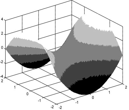
>> [X,Y]=meshgrid(-2:0.05:2);
Z=X.^2-Y.^2;
surf(X,Y,Z),shading interp,brighten(0.75),colormap(gray(5))
EXERCISE 4-1
Represent the surface defined by the equation:
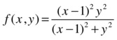
>> [x,y]=meshgrid(0:0.05:2,-2:0.05:2);
>> z=y.^2.*(x-1).^2./(y.^2+(x-1).^2);
>> mesh(x,y,z),view([-23,30])
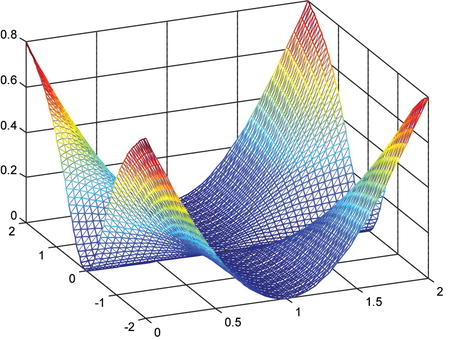
We could also have represented the surface in the following form:
>> ezsurf('y^2*(x-1)^2/(y^2+(x-1)^2)')
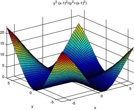
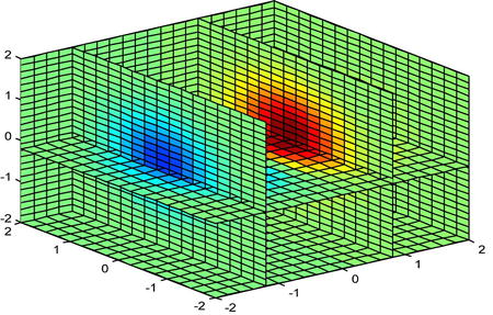
EXERCISE 4-2
Let the function f:R2Æ R be defined by:
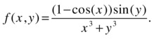
Represent it graphically in a neighborhood of (0,0).
>> [x,y]=meshgrid(-1/100:0.0009:1/100,-1/100:0.0009:1/100);
>> z=(1-cos(x)).*sin(y)./(x.^3+y.^3);
>> surf(x,y,z)
>> view([50,-15])

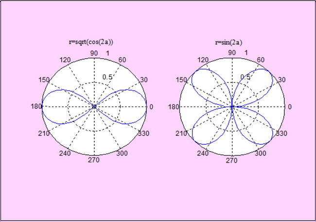
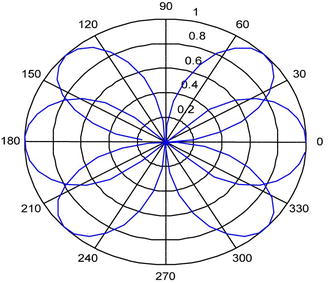
EXERCISE 4-3
Plot the following two curves, given in polar coordinates, next to each other:
![]()
Also find the intersection of the two curves.
>> a=0:.1:2*pi;
>> subplot(1,2,1)
>> r=sqrt(cos(2*a));
>> polar(a,r)
>> title('r=sqrt(cos(2a))')
>> subplot (1,2,2)
>> r=sin(2*a);
>> polar (a, r)
>> title('r=sin(2a)')
To find the intersection of the two curves, we draw them both on the same axes.
>> a=0:.1:2*pi;
>> r=sqrt(cos(2*a));
>> polar(a,r)
>> hold on;
>> r=sin(2*a);
>> polar(a,r)
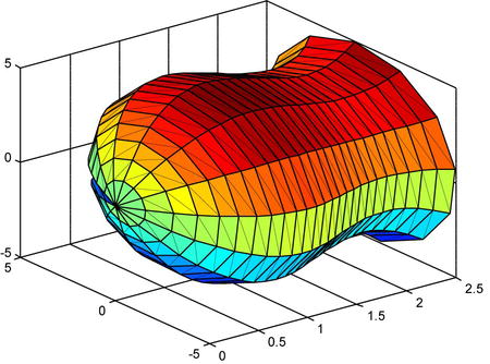
EXERCISE 4-4
Represent the surface generated by rotating the cubic ![]() around the OX axis, between the limits x = 0 and x = 5/2.
around the OX axis, between the limits x = 0 and x = 5/2.
The surface of revolution has equation ![]() , and to graph it we use the following parameterization:
, and to graph it we use the following parameterization:
![]()
>> t=(0:.1:5/2);
>> u=(0:.5:2*pi);
>> x=ones(size(u))'*t;
>> y=cos(u)'*(12*t-9*t.^2+2*t.^3);
>> z=sin(u)'*(12*t-9*t.^2+2*t.^3);
>> surf(x,y,z)
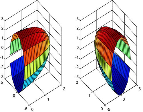
EXERCISE 4-5
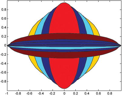
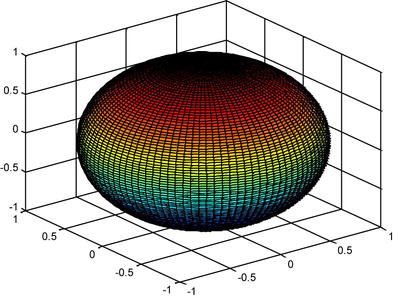
Plot the surfaces produced by rotating the ellipse  around the X axis and around the Y axis.
We represent the generated figures alongside each other, but only the positive halves of each figure. The equation of the surface of revolution around the X axis is ![]() , and is given parametrically by:
, and is given parametrically by:
![]()
The equation of the surface of revolution around the Y axis is ![]() and has the parameterization:
and has the parameterization:
![]()
>> t=(0:.1:2);
>> u=(0:.5:2*pi);
>> x=ones(size(u))'*t;
>> y=cos(u)'*3*(1-t.^2/4).^(1/2);
>> z=sin(u)'*3*(1-t.^2/4).^(1/2);
>> subplot(1,2,1)
>> surf(x,y,z)
>> subplot(1,2,2)
>> x=cos(u)'*3*(1-t.^2/4).^(1/2);
>> y=ones(size(u))'*t;
» z=sin(u)'*3*(1-t.^2/4).^(1/2);
» surf(x,y,z)
EXERCISE 4-6
Represent the intersection of the paraboloid x2 + y2 = 2z with the plane z = 2.
>> [x,y]=meshgrid(-3:.1:3);
>> z=(1/2)*(x.^2+y.^2);
>> mesh(x,y,z)
>> hold on;
>> z=2*ones(size(z));
>> mesh(x,y,z)
>> view(-10,10)
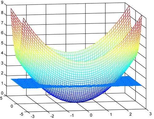
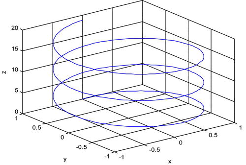
EXERCISE 4-7
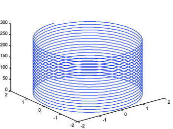
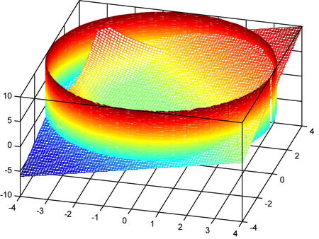
Represent the volume in the first octant enclosed between the XY plane, the plane z = x + y + 2 and the cylinder x2 + y2 = 16.
We graphically represent the enclosed volume using Cartesian coordinates for the plane and parameterizing the cylinder.
>> t=(0:.1:2*pi);
>> u=(0:.1:10);
>> x=4*cos(t)'*ones(size(u));
>> y=4*sin(t)'*ones(size(u));
>> z=ones(size(t))'*u;
>> mesh(x,y,z)
>> hold on;
>> [x,y]=meshgrid(-4:.1:4);
>> z=x+y+2;
>> mesh(x,y,z)
>> set(gca,'Box','on'),
>> view(15,45)
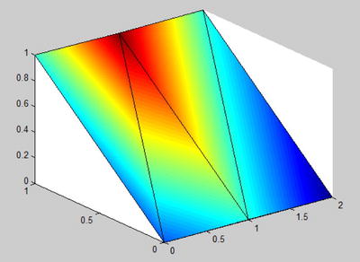
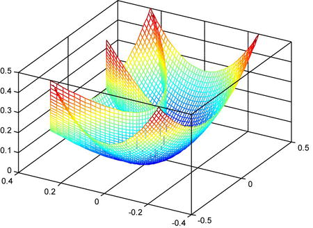
EXERCISE 4-8
Represent the volume bounded by the paraboloid x2 + 4y2 = z and laterally by the cylinders y2 = x and x2 = y.
>> [x,y]=meshgrid(-1/2:.02:1/2,-1/4:.01:1/4);
>> z=x^2+4*y.^2;
>> mesh(x,y,z)
>> hold on;
>> y=x.^2;
>> mesh(x,y,z)
>> hold on;
>> x=y.^2;
>> mesh(x,y,z)
>> set(gca,'Box','on')
>> view(-60,40)
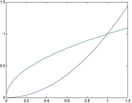
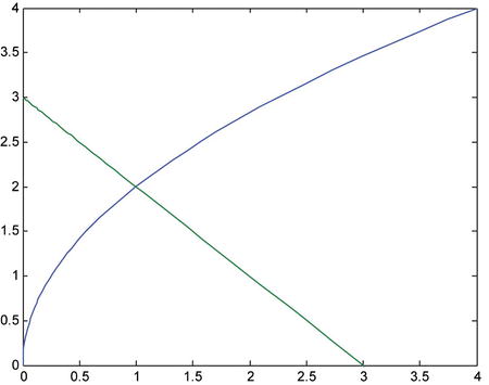
EXERCISE 4-9
Plot the parabolas y2 = x and x2 = y on the same axes. Also plot the parabola y2 = 4x and the straight line x + y = 3 on the same axes.
>> fplot('[x^2,sqrt(x)]',[0,1.2])
>> fplot('[(4*x)^(1/2),3-x]',[0,4,0,4])
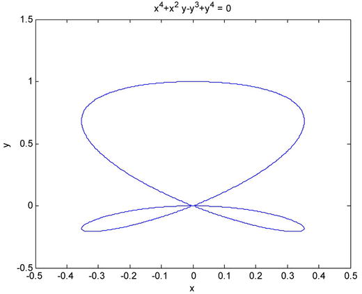
EXERCISE 4-10
Plot the curves defined by the following implicit equations:
x5 – x2y2 + y5 = 0
x4 + x2y – y5 + y4 = 0
>> ezplot('x^5-x^2*y^2+y^5', [-1,1,-1,1])
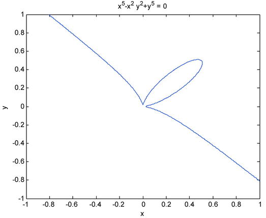
>> ezplot('x^4+x^2*y-y^3+y^4', [-1/2,1/2,-1/2,3/2])
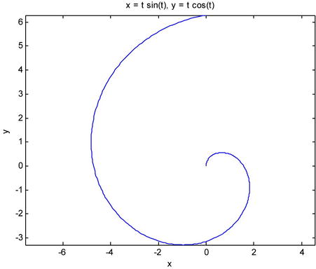
EXERCISE 4-11
Plot the curve given by the following parametric equations:
![]()
![]()
>> ezplot('t * sin(t) ',' t * cos(t)')
EXERCISE 4-12
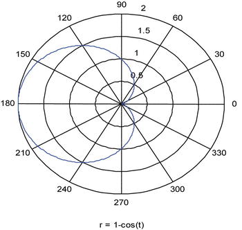
Plot the curve given by the following equation in polar coordinates:
![]()
>> ezpolar ('1 - cos (t)')