
![]()
Integration in One and Several Variables. Applications
Integrals
MATLAB includes a specially designed group of commands which allow you to work with integrals in one and several variables. The program will attempt to find primitive functions, provided they are not too algebraically complicated. In cases where the integral cannot be calculated symbolically, MATLAB enables a group of commands that allow you to approximate the integrals using the most common iterative methods.
The following table lists the most common MATLAB commands used for integration in one and several variables.
|
syms x, int(f(x), x) or int('f(x) ', 'x') |
Computes the indefinite integral >> syms x >> int((tan(x))^2, x) ans = tan(x) - x >> int('(tan(x))^2', 'x') ans = tan(x) - x |
|
int (int ('f(x,y)', 'x'), 'y')) |
Computes the double integral >> simplify(int(int('(tan(x))^2 + (tan(y))^2', 'x'), 'y')) ans = atan(tan(x)) * tan(y) - 2 * y * atan(tan(x)) + y * tan(x) |
|
syms x y, int (int (f(x,y), x), y) |
Computes the double integral >> syms x y >> simplify(int(int((tan(x))^2 + (tan(y))^2, x), y)) ans = atan(tan(x)) * tan(y) - 2 * y * atan(tan(x)) + y * tan(x) |
|
int (int (int (… int ('f (x, y…z)', 'x'), 'y')…), 'z') |
Computes the multiple integral >> int(int(int('sin(x+y+z)', 'x'), 'y'), 'z') ans = cos(x + y + z) |
|
syms x y z,. int (int (int (… int (f (x, y…z), x), y)…), z) |
Computes the multiple integral >> syms x y z >> int(int(int(sin(x+y+z), x), y), z) ans = cos(x + y + z) |
|
syms x a b, int(f(x), x, a, b) |
Computes the definite integral >> syms x >> int((cos(x))^2,x,-pi,pi) ans = PI |
|
int('f(x) ', 'x', 'a', 'b') |
Computes the definite integral >> int('(cos(x))^2','x',-pi, pi) ans = PI |
|
int (int ('f(x,y)', 'x', 'a', 'b'), 'y', ' it, ' to)) |
Computes the integral >> int(int('(cos(x+y))^2','x',-pi,pi), 'y',-pi/2,pi/2) ans = Pi ^ 2 |
|
syms x y a b c d, int (int (f(x,y), x, a, b), y, c, d) |
Computes the integral >> syms x y >> int(int((cos(x+y))^2,x,-pi,pi),y,-pi/2, pi/2) ans = pi^2 |
|
int(int(int(....int('f(x,y,…,z)', 'x', 'a', 'b'), 'y', 'c', 'd'),…), 'z', 'e', 'f') |
Computes the multiple definite integral >> int(int(int((cos(x+y+z))^2,x,-pi,pi),y,-pi/2,pi/2),z,-2*pi,2*pi) ans = 4*pi^3 |
|
syms x y z a b c d e f, int(int(int(....int(f(x,y,…,z), x, a, b), y, c, d),…), z, e, f) |
Computes the multiple definite integral >> syms x y z >> int(int(int((cos(x+y+z))^2,x,-pi,pi),y,-pi/2,pi/2),z,-2*pi,2*pi) ans = 4*pi^3 |
Indefinite Integrals, Change of Variables and Integration by Parts
The integrals whose primitive functions can be calculated symbolically, using changes of variables and integration by parts, can be directly solved using the MATLAB command int.
As a first example, we calculate the following indefinite integrals:
>> pretty(simple(int('1/sqrt(x^2+1)')))

  asinh(x)

>> pretty(simple(int('log(x)/x^(1/2)')))

     1/2
  2 x    (log(x) - 2)

>> pretty(simple(int('1/((2+x)*(1+x)^(1/2))')))

                1/2
  2 atan((x + 1)   )

>> pretty(simple(int('x^3*sqrt(1+x^4)')))

          3
          -
          2
    4
  (x  + 1)
  ---------
      6
As a second example, we calculate the following integrals by a change of variable:

>> pretty(simple(int(atan(x/2)/(4+x^2),x)))

      / x 2
  atan| - |
       2 /
  ----------
      4

>> pretty(simple(int(cos(x)^3 /sin(x)^(1/2), x)))

          1/2      2
  2 sin (x) (cos (x) + 4)
  -------------------------
              5
As a third example, we find the following integrals using integration by parts:
![]()
>> pretty(simple(int('exp(x) * cos(x) ',' x')))

   exp(x) (cos(x) + sin(x))
  ------------------------
             2

>> pretty(simple(int('(5*x^2-3)*4^(3*x+1)','x')))

   6 x           2  2                          2
  2    (90 log(2)  x  - 30 log(2) x - 54 log(2)  + 5)
  ---------------------------------------------------
                               3
                      27 log(2)
Integration by Reduction and Cyclic Integration
Integration by reduction is used to integrate functions involving large integer exponents. It reduces the integral to a similar integral where the value of the exponent has been reduced. Repeating this procedure we eventually obtain the value of the original integral.
The usual procedure is to perform integration by parts. This will lead to the sum of an integrated part and an integral of a similar form to the original, but with a reduced exponent.
Cyclic integration is similar except we end up with the same integral that we had at the beginning, except for constants. The resulting equation can be rearranged to give the original integral.
In both cases the problem lies in the proper choice of the function u(x) in the integration by parts.
MATLAB directly calculates the value of this type of integral in the majority of cases. In the worst case, the final value of the integral can be found after one to three applications of integration by parts.
As an example we find the following integral:
![]()
>> I = int('sin(x)^13 * cos(x)^15', 'x')

I =

cos(x) ^ 18/6006 - (cos(x) ^ 16 * sin(x) ^ 12) / 28 - (3 * cos(x) ^ 16 * sin(x) ^ 10) / 182 - (5 * cos(x) ^ 16 * sin(x) ^ 8) / 728 - (5 * cos(x) ^ 16 * sin(x) ^ 6) / 2002 - (3 * cos(x) ^ 16 * sin(x) ^ 4) / 4004 - (3 * cos(x) ^ 16) / 16016
Rational and Irrational Integrals. Binomial Integrals
The MATLAB command int can also be used to directly calculate the indefinite integrals of rational functions, rational powers of polynomials, binomial expressions and their rational combinations.
As an example, we calculate the following integrals:

The first integral is a typical example of a rational integral.
>> I1=int((3*x^4+x^2+8)/(x^4-2*x^2+1),x)

I1 =

3*x - (6*x)/(x^2 - 1) + atan(x*i)*i

>> pretty(simple(I1))

         6 x
  3 x - ------ + atan(x i) i
         2
        x  - 1
The second integral is a typical example of an irrational integral.
>> I2=int(sqrt(9-4*x^2)/x,x)

I2 =

3*acosh(-(3*(1/x^2)^(1/2))/2) + 2*(9/4 - x^2)^(1/2)

>> pretty(simple(I2))

         /     /  1  1/2
         |   3 | --  |    |
         |     |  2  |    |
         |      x   /    |           2 1/2
  3 acosh| - -----------  | + (9 - 4 x )
                 2       /
The third integral is a typical example of a binomial integral.
>> I3=int(x^8*(3+5*x^3)^(1/4),x)

I3 =

(5*x^3 + 3)^(1/4)*((4*x^9)/39 + (4*x^6)/585 - (32*x^3)/4875 + 128/8125)

>> pretty(simple(I3))

              5
              -
              4
        3             6        3
  4 (5 x  + 3)  (375 x  - 200 x  + 96)
  ------------------------------------
                 73125
Definite Integrals and Applications
The definite integral acquires its strength when it comes to applying the techniques of integration to practical problems. Here we present some of the most common applications.
Curve Arc Length
One of the most common applications of integral calculus is to find lengths of arcs of curve.
For a planar curve with equation y = f (x), the arc length of the curve between the points with x coordinates x = a and x = b is given by the expression:
![]()
For a planar curve with parametric coordinates x = x(t), y = y(t), the arc length of the curve between the points corresponding to the parameter values t = t0 and t = t1 is given by the expression:
![]()
For a curve given in polar coordinates by the equation r = f(a), the arc length of the curve between the points corresponding to the parameter values a = a0 and a = a1 is given by the expression:
![]()
For a space curve with parametric coordinates x = x(t), y = y(t), z = z(t), the arc length of the curve between the points corresponding to the parameter values t = t0 and t = t1 is given by the expression:
![]()
For a space curve in cylindrical coordinates given by the equations x = r·cos, y = r·sin (a), z = z, the arc length of the curve between the points corresponding to parameter values a = a0 and a = a1 is given by the expression:
![]()
For a space curve in spherical coordinates given by the equations x = r·sin (a)·cos (b), y = r·sin (a)·sin (b), z = r·cos(a), the arc length of the curve between the points corresponding to the parameter values a = a0 and a = a1 is given by the expression:
![]()
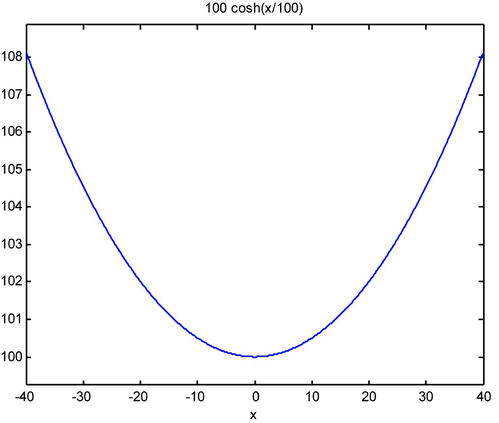
As a first example we consider a power cord that hangs between two towers which are 80 meters apart. The cable adopts the catenary curve whose equation is:
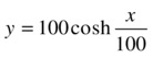
We calculate the arc length of the cable between the two towers.
We begin by graphing the catenary in the interval [– 40,40].
>> syms x
>> ezplot(100*cosh(x/100), [-40,40])
The length of the catenary is calculated as follows:
>> f=100*cosh(x/100)

f =

100*cosh(x/100)

>> pretty(simple(int((1+diff(f,x)^2)^(1/2),x,-40,40)))

           / 2
  200 sinh | - |
            5 /
If we want to approximate the result we do the following:
>> vpa(int((1+diff(f,x)^2)^(1/2),x,-40,40))

ans =

82.15046516056310170804200276894
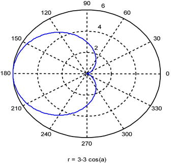
As a second example, we find the length of the cardoid defined for values from a = 0 to a = 2pi by the polar equation r = 3-3cos(a).
We graph the curve to get an idea of the length we are trying to find.
>> ezpolar('3-3*cos(a)',[0,2*pi])
Now we calculate the requested length.
>> r='3-3*cos(a)';
>> diff(r,'a')

ans =

3*sin(a)

>> R=simple(int('((3-3*cos(a))^2+(3*sin(a))^2)^(1/2)','a','0','2*pi'))

R =

24
The Area between Two Curves
Another common application of integral calculus is the calculation of the area bounded between curves.
The area between a curve with equation y = f (x) and the x-axis is given, in general, by the integral:
![]()
where x = a and x = b are the abscissas of the end points of the curve.
If the curve is given in parametric coordinates by x = x(t), y = y(t), then the area is given by the integral:
![]()
for the parameter values t = a and t = b corresponding to the end points of the curve.
If the curve is given in polar coordinates by r = f (a), then the area is given by the integral:
for the parameter values a = a0 and a = a1 corresponding to the end points of the curve.
To calculate the area between two curves with equations y = f(x) and y = g(x), we use the integral:
![]()
where x = a and x = b are the abscissas of the end points of the two curves.
When calculating these areas it is very important to take into account the sign of the functions involved since the integral of a negative portion of a curve will be negative. One must divide the region of integration so that positive and negative values are not computed simultaneously. For the negative parts one takes the modulus.
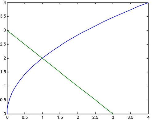
As a first example, we calculate the area bounded between the two curves: ![]() and
and ![]()
We begin by plotting the two curves.
>> fplot('[2-x^2,x]',[-2*pi,2*pi])
We need to find the points of intersection of the two curves. They are calculated as follows:

>> solve('2-x^2=x')

ans =

 -2
  1
We are now able to calculate the requested area.
>> int('2-x^2-x','x',-2,1)

ans =

9/2
As a second example, we calculate the length of, and the area enclosed by, the parameterized curves:
We begin by producing a graphical representation of the enclosed area.
>> x=(0:.1:2*pi);
>> t=(0:.1:2*pi);
>> x=cos(t).*(2-cos(2*t))./4;
>> y=sin(t).*(2+cos(2*t))./4;
>> plot(x,y)
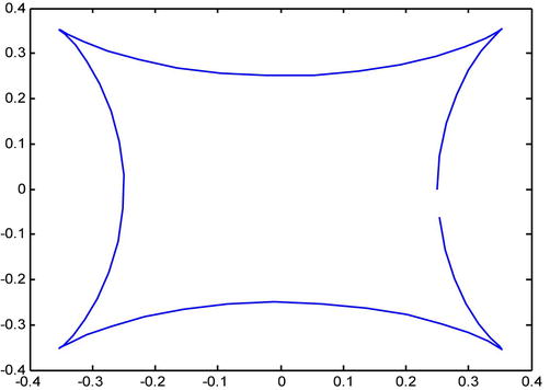
This is the figure generated as the parameter varies between 0 and 2π. We must calculate its length and the area it encloses. To avoid cancelling positive areas with negative areas, we will only work with the first half quadrant and multiply the result by 8.
For the length we have:
>> A=simple(diff('cos(t)*(2-cos(2*t))/4'))

A =

-(3*sin(t)*(2*sin(t)^2 - 1))/4

>> B=simple(diff('sin(t)*(2+cos(2*t))/4'))

B =

(3*cos(t)^3)/2 - (3*cos(t))/4

>> L=8*int('sqrt((-(3*sin(t)*(2*sin(t)^2 - 1))/4)^2+((3*cos(t)^3)/2 - (3*cos(t))/4)^2)','t',0,pi/4)

L =

3
For the area we have:
>> S=8*simple(int('(sin(t)*(2+cos(2*t))/4)*(-3/8*sin(t)+3/8*sin(3*t))', 't',0,pi/4))

S =

-(3*pi - 16)/32
As a third example, we calculate the length and the area enclosed by the curve given in polar coordinates by:
![]()
We begin by graphing the curve to get an idea of the problem.
>> a=0:.1:2*pi;
>> r=sqrt(cos(2*a));
>> polar(a,r)
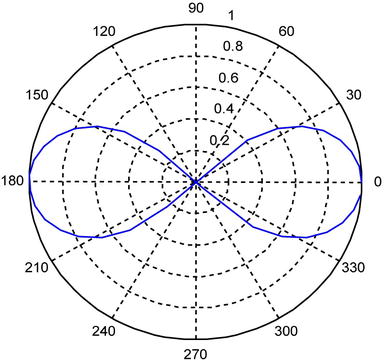
We observe that the curve repeats its structure four times as a varies between 0 and π/4. We calculate the area S enclosed by it in the following way:
>> clear all
>> syms a
>> S=4*(1/2)*int((sqrt(cos(2*a)))^2,a,0,pi/4)

S =

1
Surfaces of Revolution
The surface area generated by rotating the curve with equation y = f(x) around the x-axis is given by the integral:
![]()
in Cartesian coordinates, where x=a and x=b are the x-coordinates of the end points of the rotating curve, or
![]()
in parametric coordinates, where t0 and t1 are the values of the parameter corresponding to the end points of the curve.
The area generated by rotating the curve with equation x = f (y) around the y-axis is given by the integral:
![]()
where y = a and y = b are the y-coordinates of the end points of the rotating curve.
As a first example, we calculate the surface area generated by rotating the cubic curve 12x– 9x2+ 2x3 around the x-axis, between x = 0 and x = 5/2.
>> I=2*pi*vpa(int('(2*x^3-9*x^2+12*x)*sqrt(1+(6*x^2-18*x+12)^2)','x',0,5/2))

Warning: Explicit integral could not be found.

I =

50.366979807381457286723333012298*pi
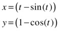
As a second example, we calculate the surface area generated by rotating the parametric curve given by x (t) = t - sin(t), y (t) = 1-cos(t) around the x-axis, between t = 0 and t = 2π.
>> clear all
>> syms t
>> x=t-sin(t)

x =

t - sin(t)

>> y= 1-cos(t)

y =

1 - cos(t)

>> V=2*pi*int(y*(sqrt(diff(x,t)^2+diff(y,t)^2)),t,0,2*pi)

V =

(64*pi)/3
The approximate area is found as follows:
>> V=vpa(2*pi*int(y*(sqrt(diff(x,t)^2+diff(y,t)^2)),t,0,2*pi))

V =

67.020643276582255753869725509963
Volumes of Revolution
The volume generated by rotating the curve with equation y = f (x) around the x-axis is given by the integral:
![]()
where x = a and x = b are the x-coordinates of the end points of the rotating curve.
The volume generated by rotating the curve with equation x = f (y) around the y-axis is given by the integral:
![]()
where y = a and y = b are the y-coordinates of the end points of the rotating curve.
If one cuts a volume by planes parallel to one of the three coordinate planes (for example, the plane z = 0) and if the equation S(z) of the curve given by the cross section is given in terms of the distance of the plane from the origin (in this case, z) then the volume is given by:
![]()
As a first example, we calculate the volumes generated by rotating the ellipse

around the x-axis and around the y-axis.
The given volumes are found by calculating the following integrals:
>> V1=int('pi*9*(1-x^2/4)','x',-2,2)

V1 =

24*pi

>> V2=int('pi*4*(1-y^2/9)','y',-3,3)

V2 =

16*pi
As a second example, we calculate the volume generated by rotating the curve given in polar coordinates by r = 1 + cos(a) around the x-axis.
The curve is given in polar coordinates, but there is no difficulty in calculating the values of x(a) and y(a) needed to implement the volume formula in Cartesian coordinates. We have:
x (a) = r (a) cos (a) = (1 + cos (a)) cos (a)
y (a) = r (a) sin (a) = (1 + cos (a)) sin (a)
The requested volume is then calculated in the following way:
>> x='(1+cos(a))*cos(a)';

>> y='(1+cos(a))*sin(a)';

>> A=simple(diff(x))

A =

- sin(2*a) - sin(a)

>> V=pi*abs(int('((1+cos(a))*sin(a))^2*(-sin(2*a)-sin(a))','a',0,pi))

V =

(8*pi)/3
Curvilinear Integrals
Let ![]() be a continuous vector field in R3 and c: [a, b] → R3 be a continuous differentiable curve in R3. We define the line integral of
be a continuous vector field in R3 and c: [a, b] → R3 be a continuous differentiable curve in R3. We define the line integral of ![]() along the curve c as follows:
along the curve c as follows:
![]()
As a first example, we consider the curve ![]() with 0 < t < 2π, and the vector field
with 0 < t < 2π, and the vector field ![]() . We calculate the curvilinear integral:
. We calculate the curvilinear integral:

>> syms t
>> pretty(int(dot([sin(t),cos(t),t],[cos(t),-sin(t),1]),t,0,2*pi))

      2
  2 pi
As a second example, we calculate the integral:
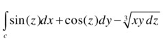
where the curve c is given by the parametric equations:
>> syms a
>> [diff(cos(a)^3),diff(sin(a)^3),diff(a)]

ans =

[ -3*cos(a)^2*sin(a), 3*cos(a)*sin(a)^2, 1]

>> int((dot([sin(a),cos(a),-sin(a)^3*cos(a)^3],[-3*cos(a)^2*sin(a), 3*sin(a)^2*cos(a),1]))^(1/3),a,0,7*pi/2)

ans =

2*(-1)^(1/3) + 3/2

>> pretty(int((dot([sin(a), cos(a) -sin(a)^3 * cos(a)^3], [- 3 * cos(a)^2 * sin(a), 3 * sin(a)^2 * cos(a), 1]))^(1/3), 0, 7 * pi/2))

        1
        -
        3   3
  2 (-1)  + -
            2

>> vpa(int((dot([sin(a), cos(a) -sin(a)^3 * cos(a)^3], [-3 * cos(a)^2 * sin(a), 3 * sin(a)^2 * cos(a), 1])) ^ (1/3), 0, 7 * pi/2))

ans =

1.7320508075688772935274463415059*i + 2.5
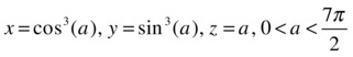
As a third example, we calculate the integral:
where c is the circle x2 + y2 = a2.
>> pretty(int('a*cos(t)^3*diff(a*sin(t),t)-a*sin(t)^3 *diff(a*cos(t),t)','t',0,2*pi))

        2
  3 pi a
  -------
     2
Improper Integrals
MATLAB works with improper integrals in the same way as it works with any other type of definite integral. We will not discuss theoretical issues concerning the convergence of improper integrals here, but within the class of improper integrals we will distinguish two types:
- Integrals with infinite limits: the domain of definition of the integrand is a half-line [(a,∞) or (-∞, a)] or the entire line (-∞,∞).
- Integrals of discontinuous functions: the given function is continuous in an interval [a, b] except at finitely many so-called isolated singularities.
Complicated combinations of these two cases may also occur. One can also generalize this to the more general setting of Stieltjes integrals, but to discuss this would require a course in mathematical analysis.
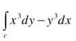
As an example, we calculate the values of the following integrals:
>> syms x a b
>> pretty(limit(int(1/sqrt(x),x,a,b),a,0))

     1/2
  2 b

>> pretty(simple(int(exp(-x)*sin(x)/x,x,0,inf)))

  PI
  --
  4
Parameter Dependent Integrals
Consider the function of the variable y : ![]() defined in the range c ≤ y ≤ e, where the function f(x, y) is continuous on the rectangle [a, b] × [c, e] and the partial derivative of f with respect to y is continuous in the same rectangle, then for all y in the range c ≤ y ≤ e:
defined in the range c ≤ y ≤ e, where the function f(x, y) is continuous on the rectangle [a, b] × [c, e] and the partial derivative of f with respect to y is continuous in the same rectangle, then for all y in the range c ≤ y ≤ e:
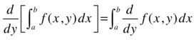
This result is very important, because it allows us to differentiate an integral by differentiating under the integral sign.
Integrals dependent on a parameter can also be improper, and in addition the limits of integration may also depend on a parameter.
If the limits of integration depend on a parameter, we have the following:

provided that a(y) and b(y) are defined in the interval [c, e] and have continuous derivatives a '(y) and b' (y), and the curves a(y) and b(y) are contained in the box [a, b] × [c, e].
Furthermore, if the function 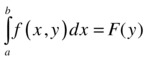 is defined on the interval [c, e] and f (x, y) is continuous on the rectangle [a, b] × [c, d], then the following holds:
![]()
i.e., integration under the integral sign is allowed and the order of integration over the variables is irrelevant.
As an example, we solve by differentiation with respect to the parameter a > 0 the following integrals:
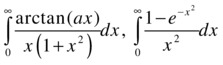
For the first integral, we will start by integrating the derivative of the integrand with respect to the parameter a, which will be easier to integrate. Once this integral is found, we integrate with respect to a to find the original integral.
>> a = sym('a', 'positive')

a =

a

>> pretty(simple(sym((int(diff(atan(a*x)/(x*(1+x^2)),a),x,0,inf)))))

    pi
  -------
  2 a + 2
Now, we integrate this function with respect to the variable a:
>> pretty(simple(sym(int(pi/(2*a+2),a))))

  pi log(a + 1)
  -------------
        2
To solve the second integral, we define:
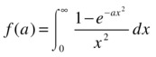
As in the first integral, we differentiate the integrand with respect to the parameter a, find the integral, and then integrate with respect to a. The desired integral is then given by setting a = 1.

>> Ia=simple(sym(int(diff((1-exp(-a*x^2))/x^2,a),x,0,inf)))

Ia =

(pi/a)^(1/2)/2

>> s=simple(sym(int(Ia,a)))

s =

(pi*a)^(1/2)
By putting a = 1, we have (1) = I(a) = ![]()
Approximate Numerical Integration
MATLAB contains functions for performing numerical integration using Simpson’s method and Lobatto’s method. The syntax of these functions is as follows:
|
q = quad(f,a,b) |
Finds the integral of f between a and b by Simpson’s method with a tolerance of 10-6 >> F = @(x)1./(x.^3-2*x-5); Q = quad(F,0,2) Q = -0.4605 |
|
q = quad(f,a,b,tol) |
Finds the integral of f between a and b by Simpson’s method with a tolerance given by tol >> Q = quad(F,0,2,1.0e-20) Q = -0.4607 |
|
q = quad(f,a,b,tol,trace) |
Finds the integral of f between a and b by Simpson’s method with tolerance tol, presenting a trace of the iteration |
|
q = quad(f,a,b,tol,trace,p1,p2,…) |
Includes extra arguments p1, p2, … for the function f, f (x, p1, p2, …) |
|
q = quadl(f,a,b) |
Finds the integral of f between a and b by Lobatto’s method with a tolerance of 10-6 >> clear all >> syms x >> f=inline(1/sqrt(x^3+x^2+1)) f = Inline function: f(x) = 1.0./sqrt(x.^2+x.^3+1.0) >> Q = quadl(f,0,2) Q = 1.2326 |
|
q = quadl(f,a,b,tol) |
Finds the integral of f between a and b by Lobatto’s method with tolerance tol >> Q = quadl(f,0,2,1.0e-25) Q = 1.2344 |
|
q = quadl(f,a,b,tol,trace) |
Finds the integral of f between a and b by Lobatto’s method with tolerance tol, presenting a trace of the iteration |
|
q = quad(f,a,b,tol,trace,p1,p2,…) |
Includes extra arguments p1, p2, … for the function f, f (x, p1, p2, …) |
|
[q,fcnt] = quadl(f,a,b,…) |
Returns the number of function evaluations |
|
q = dblquad(f,xmin,xmax, ymin, ymax) |
Finds the double integral of f (x, y) over the specified domain with a tolerance of 10-6 >> clear all >> syms xy >> z = inline(y*sin(x)+x*cos(y)) z = Inline function: z(x,y) = x.*cos(y)+y.*sin(x) >> D=dblquad(z,-1,1,-1,1) D = 1.0637e-016 |
|
q = dblquad(f,xmin,xmax, ymin, ymax, tol) |
Finds the double integral of f (x, y) over the specified domain with tolerance tol |
|
q = dblquad(f,xmin,xmax, ymin, ymax, tol, @ quadl) |
Finds the double integral of f (x, y) over the specified domain with tolerance tol using the quadl method |
|
q = dblquad(f,xmin,xmax, ymin, ymax, tol, method, p1, p2, …) |
Includes extra arguments p1, p2, … for the function f, f (x, p1, p2, …) |
As a first example, we calculate the following integral using Simpson’s method:
>> F = inline('1./(x.^3-2*x-5)'),
>> Q = quad(F,0,2)
Q =
-0.4605
Here we see that the value of the integral remains unchanged even we increase the tolerance to 10-18.
>> Q = quad(F,0,2,1.0e-18)
Q =
-0.4605
Next we evaluate the integral using Lobatto’s method.
>> Q = quadl(F,0,2)
Q =
-0.4605
Now we evaluate the double integral
>> Q = dblquad(inline('y*sin(x)+x*cos(y)'), pi, 2*pi, 0, pi)

Q =
-9.8696
Special Integrals
MATLAB provides in its basic module a comprehensive collection of special functions which help to facilitate the computation of integrals. The following table sets out the most important examples.
|
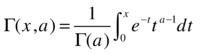
gamma(a) |
Gamma function: |
|
gammainc(x,a) |
Incomplete Gamma function |
|
gammaln(a) |
Logarithm of the gamma function Log |
|
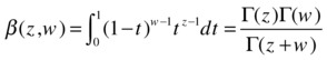
beta(z,w) |
Beta function |
|
betainc(x,z,w) |
Incomplete Beta function |
|
betaln (x,z,w) |
Logarithm of the Beta function Log β(z, w) |
|
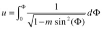
[SN,CN,DN] = ellipj(u,m) |
The Jacobi elliptic functions SN (u) = sin (φ), CN (u) = cos (φ), DN (u) = Complete elliptic functions of the 1st (k) and 2nd (e) kind |
|
k = ellipke(m) |
|
|
[k,e] = ellipke(m) |
|
|
erf (X) = error function |
F = |
|
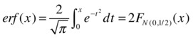
erfc(X) = complementary error function |
|
|
erfcx(X) = complementary scaled error function |
|
|
erfinv (X) = error inverse |
|
|
expint (x) |
Exponential integral |


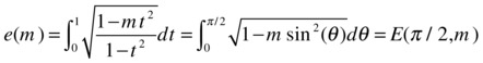
 (normal distribution)
As a first example, we calculate the normal distribution (0,1/2) for values between 0 and 1 spaced ¼ apart.
>> erf(0:1/4:1)

ans =
0 0.28 0.52 0.71 0.84
Next we calculate the values of the Gamma function at the first four even numbers.
>> gamma([2 4 6 8])

ans =
1.00 6.00 120.00 5040.00
Bearing in mind the above result we see that Γ (a) = (a-1)! for the first four even numbers.
>> [factorial(1),factorial(3),factorial(5),factorial(7)]

ans =
1.00 6.00 120.00 5040.00
Then, for z = 3 and w = 5, we find that:
- beta(z,w) = exp(gammaln(z)+gammaln(w)-gammaln(z+w))
- betaln(z,w) = gammaln(z)+gammaln(w)-gammaln(z+w)
>> beta(3,5)

ans =
0.01

>> exp(gammaln(3)+gammaln(5)-gammaln(3+5))

ans =
0.01

>> betaln(3,5)

ans =
-4.65

>> gammaln(3)+gammaln(5)-gammaln(3+5)

ans =
-4.65
Also, for z = 3 and w = 5 we check that:
beta(z,w)= Γ(z)Γ(w)/ Γ(z+w)

>> gamma(3)*gamma(5)/gamma(3+5)

ans =
0.01

>> beta(3,5)

ans =
0.01
As another example, suppose we want to calculate the length of a full period of the sinusoid y = 3sin(2x).
The length of this curve is given by the formula:
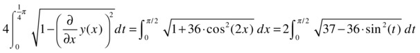
In the last step we have made the change of variable t = 2x, in addition to using cos2(t) = 1-sin2(t). The integral can now be calculated by:
>> [K,E]=ellipke(36/37)

K =
3.20677433446297
E =
1.03666851510702

>> 2*sqrt(37)*E

ans =
12.61161680006573
Definite Integrals and Applications. Several Variables
The applications of integrals of functions of several variables occupy a very important place in the integral calculus and in mathematical analysis in general. In the following sections we will see how MATLAB can be used to calculate areas of planar regions, surface areas, and volumes, via multiple integration.
Planar Areas and Double Integration
If we consider a planar region S, we can find its area through the use of double integrals. If the boundary of the region S is determined by curves whose equations are given in Cartesian coordinates, its area A is found by means of the formula:
![]()
If, for example, S is determined by a < x < b and f(x)< y <g(x) then the area will be given by:
![]()
If S is determined by h(a) < x < k(b) and c < y < d, the area will be given by:
![]()
If the region S is determined by curves whose equations are given in polar coordinates with radius vector r and angle a, its area A is given by the formula:
![]()
If, for example, S is determined by s < a <t and f (a) < r < g (a), then the area is given by:
![]()
As a first example, we calculate the area of the region bounded by the x-axis, the parabola y2 = 4x and the straight line x + y = 3.
It is convenient to begin with a graphical representation.
We see that the region can be limited to y between 0 and 2 (0 < y < 2) and for x between the curves x = y^ 2/4 and x = 3 – y. Then, we can calculate the requested area as follows:
>> A=int(int('1','x','y^2/4','3-y'),'y',0,2)

A =

10/3
As a second example, we calculate the area outside the circle with polar equation r = 2, and inside the cardioid with polar equation r = 2 (1 + cos(a)).
First of all, we graph the area of integration.
>> a=0:0.1:2*pi;
>> r=2*(1+cos(a));
>> polar(a,r)
>> hold on;
>> r=2*ones(size(a));
>> polar(a,r)
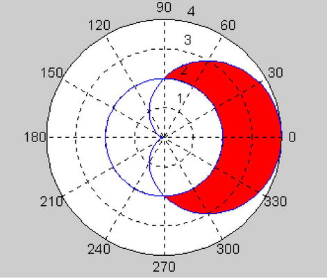
Looking at the graph, we see that, by symmetry, we can calculate half of the area by varying a between 0 and Pi/2 (0 < a Pi/2) and r between the curves r = 2 and r = 2 (1 + cos(a)):
>> pretty(int(int('r','r',2,'2*(1+cos(a))'),'a',0,pi/2))

  pi
  -- + 4
  2
The requested area is therefore 2 (π/2 + 4) = π + 8 square units.
Calculation of Surface Area by Double Integration
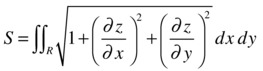
The area S of a curved surface expressed as z = f (x, y), which is defined over a region R in the xy-plane, is:
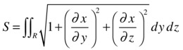
The area S of a curved surface expressed as x = f (y, z), which is defined over a region R in the yz-plane, is:
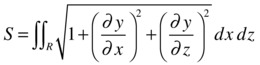
The area S of a curved surface expressed as y = f(x, z), which is defined over a region R in the xz-plane, is:
As an example, we calculate the area of the surface of the cone with equation x2 + y2 = z2, limited above the xy-plane and cut by the cylinder x2 + y2 = b y.
The projection of the surface onto the xy-plane is the region bounded by the circle with equation x2 + y2 = by, so, with MATLAB the calculation is as follows:
>> clear all
>> syms x y z a b
>> z = sqrt((x^2+y^2)/a)

z =
 ((x^2 + y^2)/a)^(1/2)

>> pretty(int(int((1 + diff(z,x)^2 + diff(z,y)^2)^(1/2), x,-(b*y-y^2)^(1/2), (b * y - y^2)^(1/2)), y, 0, b))

      2 / 1     1/2
  pi b  | - + 1 |
         a     /
  ------------------
          4
Calculation of Volumes by Double Integration
The volume V of a cylindroid with upper boundary the surface with equation z = f(x,y), lower boundary the xy-plane and laterally bounded by the cylindrical surface meeting the xy-plane orthogonally at the border of a region R, is:
![]()
The volume V of a cylindroid with upper boundary the surface with equation x = f(y,z), lower boundary the yz-plane and laterally bounded by the cylindrical surface meeting the yz-plane at the border of a region R, is:
![]()
The volume V of a cylindroid with upper boundary the surface with equation y = f(x,z), lower boundary the xz-plane and laterally bounded by the cylindrical surface meeting the xz-plane at the border of a region R, is:
![]()
As a first example, we calculate the volume in the first octant bounded between the xy-plane, the plane z = x + y + 2 and the cylinder x2 + y2 = 16.
The requested volume is found by means of the integral:
>> pretty(simple(int(int('x+y+2', 'y', 0, 'sqrt(16-x^2)'), 'x', 0, 4)))

         128
  8 pi + ---
          3
As a second example, we calculate the volume bounded by the paraboloid x2 + 4y2 = z and by the cylinders with equations y2 = x and x2 = y.
The volume is calculated using the following integral:
>> pretty(int(int('x^2 + 4 * y^2', 'y','x^2', 'sqrt(x)'), 'x', 0, 1))

  3
  -
  7
Calculation of Volumes and Triple Integrals
The volume of a three-dimensional body R, whose equations are expressed in Cartesian coordinates, is given by the triple integral:
![]()
The volume of a three-dimensional body R, whose equations are expressed in cylindrical coordinates, is given by the triple integral:
![]()
The volume of a three-dimensional body R, whose equations are expressed in spherical coordinates, is given by the triple integral:
![]()
As a first example, we calculate the volume bounded by the paraboloid ax2 + y2 = z, and the cylinder with equation z = a2 – y2 for a > 0.
The volume will be four times the following integral:
>> a = sym('a', 'positive')

a =

a

>> pretty(simple(vpa(int(int(int('1','z','a*x^2+y^2','a^2-y^2'),'y',0, 'sqrt((a^2-a*x^2)/2)'),'x',0,'sqrt(a)'))))

                                      7
                                      -
                                      2
  0.27768018363489789043849256187879 a
or, what is the same:
>> V=4*(simple(int(int(int('1','z','a*x^2+y^2','a^2-y^2'),'y',0, 'sqrt((a^2-a*x^2)/2)'),'x',0,'sqrt(a)')))

V =

(pi*(2*a^7)^(1/2))/4
As a second example, we calculate the volume bounded by the cylinders with equations z = x2 and 4 – y2 = z.
If we solve the system formed by the equations of the two surfaces we get an idea of the boundary points:
>> [x,y]=solve('x^2+0*y','4-y^2+0*x')

x =

 0
 0

y =

  2
 -2
Now we graphically represent the volume we need to calculate.
>> ezsurf('4-y^2+0*x',[-2,2],[-2,2])
>> hold on;
>> ezsurf('x^2+0*y',[-2,2],[-2,2])
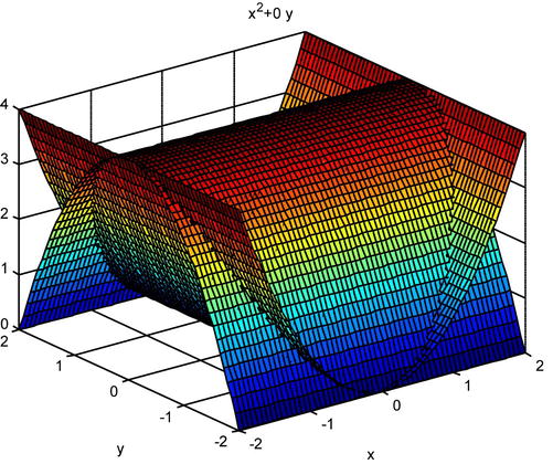
Finally, we calculate the volume as follows.
>> V=4*int(int(int('1','z','x^2','4-y^2'),'y',0,'sqrt(4-x^2)'), 'x',0,2)

V =

8 * pi
Green’s Theorem
Let C be a closed piecewise smooth simple planar curve and R the region consisting of C and its interior. If f and g are continuous functions with continuous first partial derivatives in an open region D containing R, then Green’s theorem tells us that:
As an example, using Green’s theorem, we calculate the integral:
![]()
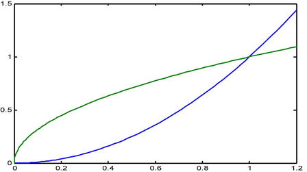
where C is the boundary of the region enclosed by the parabolas y = x2 and x = y2.
The two parabolas intersect at the points (0,0) and (1,1). This gives us the limits of integration.
>> clear all
>> fplot('[x^2,sqrt(x)]',[0,1.2])
We can now calculate the integral:
>> syms x y
>> m = x + exp(sqrt(y))

m =

x + exp(y^(1/2))

>> n = 2 * y + cos(x)

n =

2*y + cos(x)

>> I = vpa(int(int(diff(n,x)-diff(m,y), y, x^2, sqrt(x)), x, 0, 1))

I =

-0.67644120041679251512532326651204
The Divergence Theorem
Suppose Q is a domain with the property that each straight line passing through a point inside the domain cuts its border at exactly two points. In addition, suppose the boundary S of the domain Q is a closed piecewise smooth oriented surface with outward pointing unit normal n on the boundary. If f is a vector field that has continuous partial derivatives on Q, then the Divergence Theorem tells us that:
![]()
The left-hand side of the former equality is called the outflow of the vector field f through the surface S.
As an example, we use the divergence theorem to find the outflow of the vector field f = (xy + x2y z, yz + xy2 z, xz + xyz2) through the surface of the cube defined in the first octant by the planes x = 2, y = 2 and z = 2.
>> clear all
>> syms x y z
>> M = x * y + x ^ 2 * z * y

M =
y * z * x ^ 2 + y * x

>> N = y * z + x * y ^ 2 * z

N =
 x * z * y ^ 2 + z * y

>> P = x * z + x * y * z ^ 2

P =
x * y * z ^ 2 + x * z

>> simple Div = (diff(M,x) + diff(N,y) + diff(P,z))

Div =

x + y + z + 6 * x * y * z

>> I = int(int(int(Div,x,0,2), y, 0, 2), z, 0, 2)

I =

72
Stokes’ Theorem
Suppose S is an oriented surface of finite area defined by a function f(x,y), with boundary C having unit normal n. If F is a continuous vector field defined on S, such that the function components of F have continuous partial derivatives at each non-boundary point of S, then Stokes’ Theorem tells us:
![]()
As an example, we use Stokes’ theorem to evaluate the line integral:
![]()
where C is the intersection of the cylinder x2 + y2 = 1 and the plane x + y + z = 1, and the orientation of C is counterclockwise in the xy-plane.
The curve C bounds the surface S defined by z = 1–x–y = f(x,y) for (x, y) in the domain D = {(x,y) / x2 + y2 = 1}.
We put F= – y3 i + x3 j – z3 k.
Now we calculate rot(F) and find the above integral over the surface S.
>> F = [- y ^ 3, x ^ 3, z ^ 3]

F =

[- y ^ 3, x ^ 3, z ^ 3]

>> clear all
>> syms x y z
>> M = - y ^ 3

M =

- y ^ 3

>> N = x ^ 3

N =

x ^ 3

>> P = z ^ 3

P =

z ^ 3

>> rotF=simple([diff(P,y)-diff(N,z),diff(P,x)-diff(M,z),diff(N,x)-diff(M,y)])

rotF =

[0, 0, 3 * x ^ 2 + 3 * y ^ 2]
Therefore, we have to calculate the integral ∫D (3 x2+ 3 y2) dx dy. Changing to polar coordinates, this integral is calculated as:
>> pretty (simple (int (int('3*r^3', 'a',0,2*pi), 'r', 0, 1)))

  3 pi
  ----
   2
EXERCISE 8-1
Calculate the following integrals:
![]()
>> pretty(simple(int('sec(x)*csc(x)')))
log(tan(x))
>> pretty(simple(int('x*cos(x)')))
cos(x) + x sin(x)
>> pretty(simple(int('acos(2*x)')))
2 1/2
(1 - 4 x )
x acos(2 x) - -------------
2
EXERCISE 8-2
Find the following integrals:
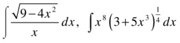
>> pretty(simple(int('(9-4*x^2)^(1/2)/x')))
/ / 1 1/2
| 3 | -- | |
| | 2 | |
| x / | 2 1/2
3 acosh| - ----------- | + (9 - 4 x )
2 /
>> pretty(simple(int('x^8*(3+5*x^3)^(1/4)')))
5
-
4
3 6 3
4 (5 x + 3) (375 x - 200 x + 96)
------------------------------------
73125
EXERCISE 8-3
Find the following integrals: a = ![]() and b =
and b = ![]()
We have a = Γ (4).
Making the change of variable x3 = t we see that b =  = Γ (1) / 3.
Therefore, for the calculation of a and b we will use the following MATLAB syntax:
>> a = gamma(4)
a =
6
>> b = (1/3) * gamma(1)
b =
0.3333
EXERCISE 8-4
Solve the following integrals:
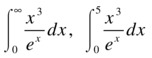
As ![]() , the first integral is solved as:
, the first integral is solved as:
>> gamma (4)
ans =
6
As 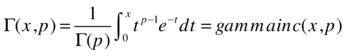 , the second integral is solved as follows:
>> gamma(4) * gammainc(5.4)
ans =
4.4098
EXERCISE 8-5
Solve the following integrals:
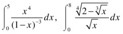
![]() and
and 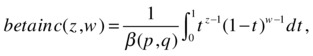 which means the first integral is solved as:
>> beta (5,4) * betainc(1/2,5,4)
ans =
0.0013
For the second integral, we make the change of variable x1/3 = 2t, so the integral becomes the following:
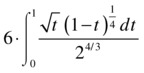
whose value is calculated using the MATLAB expression:
>> 6 * 2 ^(3/4) * beta(3/2,5/4)
ans =
5.0397
EXERCISE 8-6
Find the value of the following integrals:
 and
and 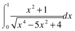
Via a change of variable one can convert such integrals to standard elliptic integrals. MATLAB enables symbolic functions that calculate the values of elliptic integrals of the first, second and third kind.
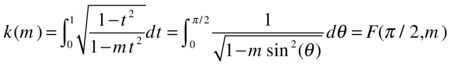

The function [k, e] = ellipke(m) estimates the two previous integrals.
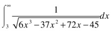
For the first integral of the problem, as the subradical polynomial is of degree 3, we make the change of variable x = a + t2, a being one of the roots of the subradical polynomial. We take the root x = 3 and make the change x = 3 + t2, with which we obtain the integral:
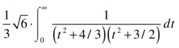
Now we make the change of variable t = (2/√3) tan(u), so the integral transforms into the full elliptic integral of the first kind:
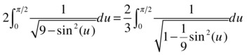
whose value is calculated using the expression:
>> (2/3) * ellipke(1/9)
ans =
1.07825782374982
For the second integral we put x = sin t and we get:
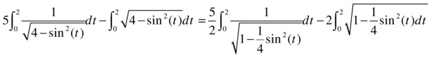
We have reduced the problem to two elliptic integrals, the first of the first kind and the second of the second kind, whose values can be calculated using the expression:
>> [K, E] = ellipke (1/4)
K =
1.68575035481260
E =
1.46746220933943
>> I = (5/2) * K-2 * E
I =
1.27945146835264
EXERCISE 8-7
Calculate the length of a full period of the sinusoid y = 3sin(2x).
The length of this curve is given by the formula:
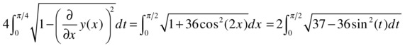
In the last step, we have made the change of variable 2x = t, using in addition cos2(t) = 1 - sin2(t). The value of the integral can be calculated now by:
>> [K, E] = ellipke (36/37)
K =
3.20677433446297
E =
1.03666851510702
>> 2 * sqrt (37) * E
ans =
12.61161680006573
EXERCISE 8-8
Calculate the integral 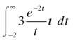
This is an exponential type integral. We make the change of variable v = 2t and obtain the equivalent integral:

which is calculated via the MATLAB expression:
>> 3 * expint(-4)
ans =
-58.89262341016866 - 9.42477796076938i
The solution would normally be taken to be the real part of the previous result.
EXERCISE 8-9
Calculate the area bounded by the curve ![]() and the x-axis.
and the x-axis.
We begin by graphing the area.
>> fplot('[x^3-6*x^2+8*x,0]',[-1,5])
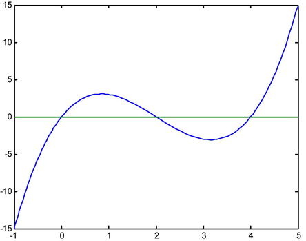
The points where the curve cuts the x-axis are (0,0), (0,2) and (0,4), as we see by solving the following equation:
>> solve('x^3-6*x^2+8*x')
ans =
0
2
4
As there is both a positive region and a negative region, the area is calculated as follows:
>> A = abs(int(x^3-6*x^2+8*x,0,2)) + abs(int(x^3-6*x^2+8*x,2,4))
A =
8
EXERCISE 8-10
Calculate the area bounded between the parabolas ![]() and
and ![]() .
.
We begin by plotting the area.
>> fplot('[6*x-x^2,x^2-2*x]',[-1,7])
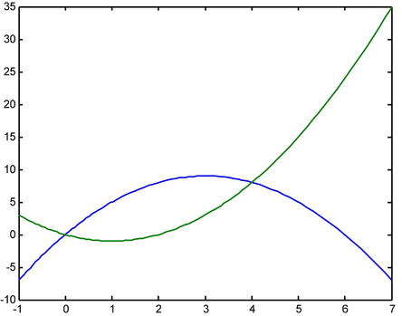
We find the points of intersection of the two curves:
>> [x, y] = solve('y=6*x-x^2,y=x^2-2*x')
x =
0
4
y =
0
8
The points of intersection are (0,0) and (4,8).
The area is then calculated as follows:
>> A = abs(int('(6*x-x^2)-(x^2-2*x)',0,4))
A =
64/3
EXERCISE 8-11
Calculate the area enclosed by the three rose petals defined in polar coordinates by ![]() .
.
We begin by graphing the curve.
>> ezpolar('5*cos(3*a)')
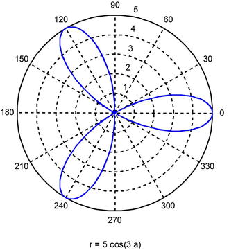
The total area can be calculated by multiplying by 6 the area as a ranges between 0 and π/6 (the upper half of the horizontal petal). We will then have:
>> A=6*int((1/2)*5^2*cos(3*a)^2,0,pi/6)
A =
(25*pi)/4
EXERCISE 8-12
Calculate the area between the x-axis and the full arc of the cycloid with parametric equations:
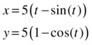
where t ranges between 0 and 2π.
The requested area is given by the integral:
>> A=int(5*(1-cos(t))*diff(5*(t-sin(t))),0,2*pi)
A =
75*pi
EXERCISE 8-13
Calculate the volumes generated by rotating the curve y = sin(x) around the x-axis and around the y-axis on the interval [0,π]
>> Vox=pi*int('sin(x)^2',0,pi)
Vox =
pi^2/2
>> Voy=2*pi*int('x*sin(x)',0,pi)
Voy =
2*pi^2
EXERCISE 8-14
Calculate the volume generated by rotating around the y-axis the arc of the cycloid with parametric equations:
where t varies between 0 and 2π.
The requested volume is given by the integral:
>> V=2*pi*int('(t-sin(t))*(1-cos(t))*(1-cos(t))',0,2*pi)
V =
6*pi^3
EXERCISE 8-15
Calculate the volume generated by rotating the polar curve
![]()
around the x-axis. We first plot the curve:
>> ezpolar('2*sin(a)')
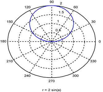
We note that the integral will be given by varying the angle between 0 and π. By symmetry, we can calculate the result by doubling the corresponding volume generated for the angle between 0 and π/2.
The volume is then calculated by the following integral:
>> V=2*2*pi/3*int((2*sin(a))^3*sin(a),0,pi/2)
V =
2*pi^2
EXERCISE 8-16
Calculate the length of the curve:
![]()
as x varies between 0 and 2.
The length is calculated directly by the following integral:
>> L=int((1+(diff('2*x*sqrt(x)'))^2),0,2)
L =
20
EXERCISE 8-17
Calculate the length of the astroid:
![]()
The curve can be expressed parametrically as follows:
We now represent the astroid to find the limits of variation of the integral.
>> ezplot('2*cos(t)^3','2*sin(t)^3')
Looking at the graph we can see that the integral can be found by multiplying by 4 the length obtained as the parameter varies between 0 and π/2.
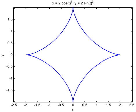
The length of the astroid is calculated by the following integral:
>> L=4*int(((diff('2*cos(t)^3'))^2+(diff('2*sin(t)^3'))^2)^(1/2),0,pi/2)
L =
12
EXERCISE 8-18
Calculate the integral:
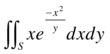
where S is the planar region bounded by x = 0, y = x2+1 and y = 2.
The region S is determined by 1< y <2 and 0< x <y1/2.
The integral is calculated as follows:
>> int(int('x*exp(-x^2/y)','x',0,'sqrt(y)'),'y',1,2)
ans =
3/4 - 3/(4*exp(1))
EXERCISE 8-19
Calculate the volume enclosed between the two cylinders:
z = x2 and z = 4 – y2.
The problem is solved by calculating the integral:
>> 4*int(int(int(1,z,x^2,4-y^2),y,0,sqrt(4-x^2)),x,0,2)
ans =
8*pi
EXERCISE 8-20
Calculate the integral:
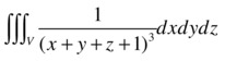
where V is the volume enclosed between the three coordinate planes and the plane x + y + z = 1.
The body V is determined by:
0 < x < 1, 0 < y < 1 - x, 0 < z < x - y
The integral that solves the problem is the following:
>> x=sym('x','positive')
x =
x
>> vpa(int(int(int(1/(x+y+z+1)^3,z,0,1-x-y),y,0,1-x),x,0,1))
Warning: Explicit integral could not be found.
ans =
0.034073590279972654708616060729088