
Now that you have an understanding of the hands-on digital audio editing tools in Audacity, it’s time to look at how you can use algorithms, which take the form of plug-in filters and effects, to apply waveform editing operations and special effects with math and code routines.
You’ll look at a number of the primary audio editing and “sweetening” effects in the Audacity 2.1 Effect menu. Some of them visualize the concepts that you learned about in the first few chapters of the book. This offers reinforcement of the principles. You will learn how to utilize algorithms that allow you to amplify waveforms, shift the pitch, change the playback speed, equalize the frequency response, and apply audio effects such as reverb and echo (delay). You also learn how to selectively filter frequencies out of your sample waveform by using audio filters such as High Pass, Low Pass, and Notch Filters.
Audacity 2.1 has 44 default Effect menu entries, so I can’t cover them all in this chapter. I’ll cover the ones that demonstrate the concepts you have already learned, and some of the others that are editing mainstays; so you’ll learn all the basic processing.
It’s important to note that there are another 80 plug-in filters that you can add to the Effect menu by using Effect ➤ Manage, shown at the top of the Effect menu in Figure 8-1.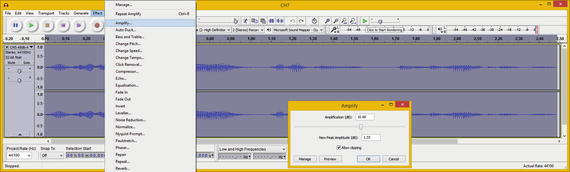
Figure 8-1.
Select sample and use an Effect ➤ Amplify algorithm
Algorithmic Audio Effects Processing
Algorithms are code (usually C++ in digital audio editing) that process your sample waveform. This is why it is important that you use a high-quality sampling frequency—at least CD quality (44.1 kHz) or THX quality (48 kHz)—and leave the sample resolution at 32 bits until the editing and processing is done and you are ready to perform data footprint optimization.
The reason for using the highest possible sampling frequency and sample resolution is that you want to give as much data to the algorithm as you possibly can. The more data the algorithm has, the better results it can provide. Later, after all the processing is complete, you can reduce your sample resolution to 24-bit (HD), or more likely to 16-bit, which is CD quality. You can preview using your ears, your eyes (waveform), and even a data result (export audio as PCM or FLAC), as you’ve seen in previous chapters and will see in this chapter.
Waveform Amplitude: The Amplify Effect
The first effect that you apply increases the y-axis dimension in the amplitude of the waveform. The result of this is amplification, more commonly referred to as “turning up the volume.” Open your CH7.aud Audacity project and select the entire waveform, as is shown in Figure 8-1. Select Effect ➤
Amplify
and enter an amplification factor in decibels; I used 10.6, which is a 133% peak amplitude (a 1.33 factor). Next, select the Allow clipping option. You can also use the Preview button to preview different settings until you find one that sounds good to you.
Once you click the OK button to apply an Amplify effect, you are able to see this effect algorithmically applied to your waveform. This is shown in Figure 8-2, and as you can see, the waveform looks (and sounds) drastically different.
Figure 8-2.
Amplitude y-axis dimension of waveform is magnified
The sample is indeed louder on playback; however, as you can hear, the quality is lower. I don’t hear any artifact introduction, but the clarity of the vocals has suffered, so I used the Edit ➤ Undo Amplify menu sequence to undo the algorithm processing. I will tell my app users to turn up their volume.
If you look at the amplified data sample waveform shown in Figure 8-2, it is obvious that this sample waveform has been stretched (only) along the y axis, which is the amplitude (volume) of your sample. This effect reinforces what you learned about audio sample characteristics in Chapter 3.
Next, let’s take a look at the x axis, or frequency, of the waveform. Changing the frequency of your waveform is called pitch shifting.
Waveform Frequency: The Pitch Shifting Effect
Next, let’s take a look at the other sample characteristic that you learned about in Chapter 3, sample frequency. To change your data sample frequency, you use the Effect ➤ Change Pitch menu sequence, which is shown on the left side of Figure 8-3. I shifted the pitch up one octave, or 100%, so that my vocal sounds like a member of the popular chipmunk trio.
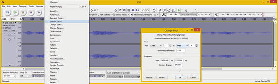
Figure 8-3.
Select sample, then Effect ➤ Change Pitch algorithm
As you can see in the Change Pitch dialog, there are 12 semitones to an octave, and the Percent Change data field shows that there is a 100% full octave pitch increase indicated.
If you are sampling notes using an instrument that is in tune, you can also select pitch changes by notes. I clicked the OK button to apply the algorithm. This time, the x axis of the sampled waveform was affected and the amount of data was doubled in this dimension, creating a waveform twice as dense, as you can see in Figure 8-4.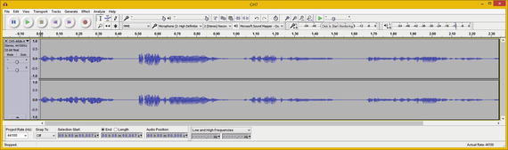
Figure 8-4.
Frequency x-axis dimension of sample is compressed
Since I’m not currently working on a chipmunks movie or games, I used the Edit ➤ Undo Change Pitch menu sequence to return to the original data sample waveform.
Waveform Speed: Vinyl Record Playback Speeds
An algorithm similar to the Change Pitch effect is the Change Speed effect (see Figure 8-5). It does much the same thing to your frequency (the x axis) without keeping the sample length (time) the same. What this does is shorten the (time) length for your sample. Interestingly, the paradigm that the Change Speed dialog uses is old-fashioned vinyl record RPMs! The baseline is large 33.3 RPM records with options to change the playback speed to match a 45 RMP record, or even an ancient 78 RPM record. As you can see, the dialog also allows you to specify speed adjustment using a multiplier, percentage, or actual time value, all of which are calculated in real time.
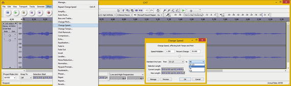
Figure 8-5.
Select sample, then Effect ➤ Change Speed algorithm
As you can see in Figure 8-6, your data sample waveforms are compressed along the x axis like they were in Change Pitch, but the sample is shorter (rather than length being maintained), as you can see on the right. This 35% change is the amount of gray shown on the right in Figure 8-6; you can see the multiplier and percent change numbers that you specified in the dialog visually inside the Audacity 2.1.1 application.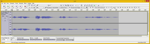
Figure 8-6.
Frequency x axis and length of sample is compressed
Next, let’s look at one of the more complex algorithms, Equalization; it has a more detailed user interface. This effect is a lot of fun to tweak, and with a visual UI, it is fairly easy to use. Equalization is one of the more popular audio effects among consumers, as is evidenced by the large numbers of stereos that come equipped with equalization sliders.
Waveform Equalization: The Equalization Algorithm
If you want to equalize your digital audio sample, you can use the Audacity Equalization (EQ) effect
. It permanently applies an EQ setting to your audio data, so make sure that no one else plans to put their EQ settings on top of yours! As you can see in Figure 8-7, the dialog for this effect can be very involved.
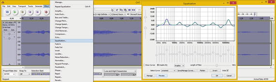
Figure 8-7.
Select sample, then Effect ➤ Equalization algorithm
The easiest (and most familiar) mode in the user interface is the Graphic EQ mode. Select the Graphic EQ radio button and let the Equalization dialog draw the curves for you, as shown in Figure 8-7.
As you can see, the Equalization dialog is very powerful. It offers fine-tuned adjustment of any frequency. You can add to or subtract from any of 32 different frequencies.
The best way to work with this effect is to use your ears to preview your slider settings as frequently as you can. This is made easy with the Preview button, shown highlighted in blue in the lower left of the dialog shown in Figure 8-7.
The two sliders on the left, as well as the Length of Filter slider on the bottom of the dialog, allow you to fine-tune the frequency grid display that the spline curves will be drawn on top of. If you want to learn more about spline curves, check out my Android Studio New Media Fundamentals (Apress, 2015) book; it covers the fundamentals of all five of the new media genres.
You can save equalization curve collections with presets by using the Save/Manage Curves feature. You can invert or flatten your curves by using the Flatten and Invert buttons. You’ll find you can also turn off the grid guidelines by deselecting the Grids check box, although I recommend that you keep them visible.
Waveform Reverberation: The Reverb Effect
Another popular digital audio effect that is often applied with algorithmic processing is reverb. Reverb
simulates being inside an enclosure, whether a small room or a large amphitheater. For this reason, a primary setting in the Reverb dialog (see Figure 8-8) is the Room Size, which defaults to 75%. There’s also a millisecond pre-delay data value that you can provide, as well as Reverberance, Damping, and Stereo Width percentage values. To fine-tune the effect, you can reduce the percentage of low tone and high tone frequencies that get through the filter, and set custom Wet Gain or Dry Gain values in decibels.
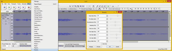
Figure 8-8.
Select sample, and select Effect ➤ Reverb algorithm
I decided to try the default settings, which provide a standard reverb processing result, to see what the algorithmic processing is going to do to a sample waveform.
As you can see in Figure 8-9, the sample waveform is far more complex than it was before. This means that an effect like reverb is going to influence your data footprint, because there is more data to compress. The areas that were silent (thin lines) have room echo data in them, as you can see over the duration of the entire data sample.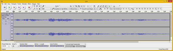
Figure 8-9.
Frequency x axis and length of sample is compressed
Therefore, if your application doesn’t require reverb as a special effect, or more importantly, if the platform that you will deliver on can add that effect to the waveform (like Java and Android), then you do not want to “hard-code” the data inside of your basic sample waveform. This approach allows you to have more flexibility in manipulating audio inside of an application. The core effects that you’re looking at in this chapter are available in many open source new-media platform API packages, such as those in Java, JavaFX, and Android Studio.
Next, let’s look at another effect that provides the echo processing framework to audio waveforms, the Delay effect.
Waveform Echo Chamber: The Delay Effect
Whereas the Reverb effect
is a subtle type of echo effect, you can create more pronounced echo effects that are more like the long distance echo effects you get in canyons, for instance, by using the Delay effect. There are several types of delay, such as a regular bouncing ball or a reverse bouncing ball, in the Delay drop-down menu (see Figure 8-10). You can set the delay level and the delay time, and even set a pitch change effect from Pitch/Tempo to Pitch Shift. You can fine-tune this effect by specifying the pitch change for each echo using semitones (as you did in the Change Pitch effect) and the number of echoes to produce.
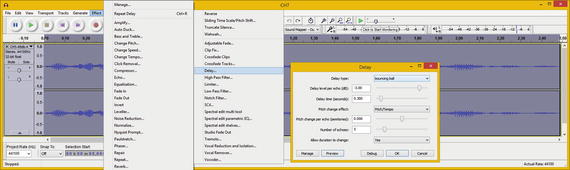
Figure 8-10.
Select sample, and select Effect ➤ Delay algorithm
As you can see, I selected the bouncing ball delay type, because I like the delay signature that I hear when I bounce a ball. As you might imagine, this delay effect extends your sample duration because it is adding significant echo data (see Figure 8-11). The black vertical line on the right is the end of what was the original sample length. The more delay time and the higher the number of echoes that you specify, the longer the new data sample (time) length becomes.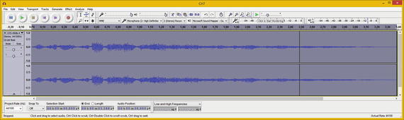
Figure 8-11.
The Delay effect may extend the data sample length
The Delay effect can add more to the data footprint of a sample than the Reverb effect, so make sure that you need to add echo into your sample; otherwise, find a way to process it “externally” by using Java code, or even OS or hardware capabilities that may provide EQ, reverb, and echo.
Next, let’s take a look at how to “shave” frequencies off of your data sample. This is usually done with the Low Pass and the High Pass Filters. You’ll use the Low Pass Filter to remove the last remnants of those chirping artifacts you’ve worked with in the past few chapters. If that doesn’t work, there’s also a Notch Filter that allows you to target (notch) individual frequencies that you want to filter out or remove from the sample frequency spectrum.
Waveform Shaving: The Low Pass Filter Effect
The High Pass Filter and the Low Pass Filter
remove unnecessary frequency data, or frequency data that’s undesirable or causing problems with your intended aural result. It can be a good data footprint optimization tool, because even a frequency that cannot be heard needs to be encoded as data, which means that these filters can be used to remove sample data that is not needed (or heard), and thus reduce the data footprint.
As you can see in Figure 8-12, this dialog allows you to specify the Cutoff frequency, where everything lower (Low Pass) or higher (High Pass) is “shaved” or removed from the frequency spectrum by the filter’s algorithm. There’s also the Rolloff setting, which specifies the number of decibels per octave that the filter is going to affect. This specifies a magnitude for the application of your cut-off frequency value.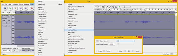
Figure 8-12.
Select sample, and select Effect ➤ Low Pass Filter
My process for trying to use the Low Pass Filter to remove the last remnants of the chirp artifact was to first use Audacity’s default Low Pass Filter settings of 6 dB and 1000 Hz.
This affected the vocal sample and made it duller, so I increased the default cut-off frequency to brighten the vocal sample back up to where it was, while lessening the final remnants of the chirp artifact.
This value turned out to be a value of 2000 Hz, because higher values permitted the remaining chirp artifact to make it through this tonal filter.
After I ascertained the optimal cut-off frequency setting to use, I selected a 12 dB Rolloff option. This provided chirp removal, but it did not affect the vocal data sample quality much.
Finally, I tried a setting of 24 dB, which affected the quality of the vocal part of my data sample too much; so, the final settings for the Low Pass Filter effect were 12 dB and 2000 Hz.
Next, let’s take a look at the more surgical Notch Filter, which allows you to specifically target any frequency.
Tunneling Into Your Waveform: The Notch Filter
Instead of cutting off the top or bottom sample waveform frequencies, the Notch Filter effect
allows you to surgically “tunnel” into any section of your sample to remove a specific frequency or a range surrounding that frequency. As you can see in Figure 8-13, the Notch Filter dialog allows you to specify your target Frequency and Q value, which is the tunnel width around that frequency. Lower Q values make this tunnel smaller, and so a very small Q value essentially targets the frequency with more surgical precision. The default settings are 60 Hz and a 1.0 Q factor, which I need to change to find the frequencies of the remaining chirp artifacts.
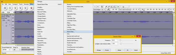
Figure 8-13.
Select sample, and select Effect ➤ Notch Filter
My process for finding the frequency was to use the Preview button, first at 60 Hz and then at the maximum of 10000 Hz, where the artifact was still audible. Then I used a halfway mark of 5000 Hz, and then backed off that in increments of 1000 until I hit two frequencies that the artifacts were not audible at. These were 3000 Hz and 4000 Hz. I decided to use 4000 Hz because the result sounded better. I left the 100% tunnel size, as you can see in Figure 8-14, and clicked the OK button to apply.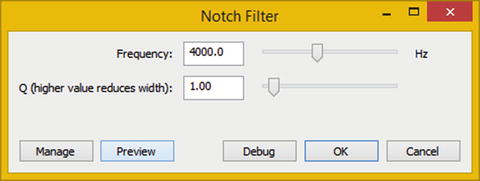
Figure 8-14.
Setting the Notch Filter to a Frequency of 4000 Hz
To see the amount of data that the Notch Filter removed, I targeted the chirp artifact. Then I saved the data sample using the FLAC file format. As you can see in Figure 8-15, the file size is now 104 KB, whereas before it was 112 KB. So, the Notch Filter removed 8 KB worth of artifact data from the sample. The file size is now more than 300% less (104 KB × 3 = 312 KB). The original unedited baseline FLAC file was 316 KB.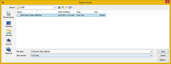
Figure 8-15.
This sample now has over 300% less data footprint
If the FLAC format is getting a 104 KB data footprint for this audio data sample, other data formats will provide an even smaller data footprint, as you will see in chapter covering data footprint optimization.
Summary
In this chapter, you looked at digital audio processing using algorithms found in the Audacity Effect menu, where internal effects and plug-in filters can be accessed. You looked at many of the mainstream digital audio editing effects that are applied when editing and sweetening digital audio samples. These effects include Amplify, Pitch Shifting, Sample Speed, Equalization, Reverb, Delay, Low Pass Filter, and Notch Filter. You also looked at the Effect ➤ Manage menu sequence, which accesses a dialog that allows you to see the other 80 plug-in filters that are not on the Effect menu. Be sure to familiarize yourself with all 128 plug-in filters on the Audacity Effect menu if you want to become a digital audio editing professional.
In the next chapter, you learn about digital audio data visualization, by using spectral analysis concepts, terms, and principles, along with the Audacity 2.1.1 Analyze menu.