
Now that you know the general history of digital audio, it is time to get into digital audio sampling (essentially the same as digital audio recording), which needs to be done before any digital audio editing can be done. This chapter covers the concepts behind “digitizing” analog audio—or turning it into digital audio—by defining which sampling frequency is utilized during the digitization process and which sample resolution is used to store individual samples of analog audio waveforms as digital audio data.
In addition to digital audio sampling concepts, such as sampling frequency and sample resolution
, you also look at standard sampling frequencies and sample resolutions, which are used in the digital audio industry, and how to sample, or record, digital audio by using Audacity 2.1.1 for Windows.
Data Sampling: Resolution and Frequency
In this chapter, I cover the process of digital audio
data sampling
. You will see how the transition can be made between analog audio and digital audio using the process of sampling, which you are already familiar with if you do sound design and music synthesis.
Sampling is even discussed in the news, as recording artists are sometimes sued for taking little “riffs” or “snippets” of another artist’s song and sampling it in their songs. For this reason, be very careful with what you are sampling; make sure that it is an original analog audio waveform or that you have permission to use it! I want to make sure that you have a firm understanding of the digital audio new media assets that you will eventually create, optimize, and “render” via open source APIs, such as Java and JavaFX, or the Android Studio digital audio playback classes, SoundPool and MediaPlayer.
Sampling Digital Audio : Taking a Data Sample
The process of turning analog audio (sound waves) into digital audio data is called sampling. If you work in the music industry, you have probably heard about a type of keyboard (or rack-mount equipment) called a “sampler.” Specifically, sampling is the process of slicing an audio wave into segments so that you can store the shape of that wave as digital audio sample data, which is later reproduced using a hardware device with digital audio support. The sample data can be stored by using a codec and digital audio file format, which is discussed in Chapter 4.
Audio data sampling turns infinitely accurate analog sound waves into discreet (finite) digital audio data; that is, into a collection of zeroes and ones, often called
binary data
.
The more zeroes and ones that are used, the more infinitely accurate the reproduction of the original analog sound wave will be. The sample accuracy determines the number of zeroes and ones that are used to reproduce an analog sound wave; these sample accuracy topics are covered next.
Data Sample Resolution: Data Bytes per Sample
Each digital slice of your sampled audio sound wave is called a sample because it takes a sampling of your sound wave at an exact point in time. The precision, or resolution, of each sample is determined by the amount of data that is utilized to define each wave slice height, or the amplitude. Just as with digital imaging, this precision is termed the
resolution
, or more accurately (no pun intended), your digital audio waveform sample resolution.
It is important to remember that digital audio resolution
takes samples along the amplitude of your audio waveform, which takes place along the y axis of the audio sample waveform (if you are looking at the data using a 2D representation). This is shown in Figure 3-1, where the amplitude is measured by the height of the waveform; in this case, it is a simple sine wave used for visualization purposes. You may have learned about sine waves in school. Simple tones can be produced by audio oscillator hardware using sine waves, as you will see in the more advanced chapters of the book when you use the Audacity Generate menu to create waveforms algorithmically. In Chapter 5, you begin a lot of hands-on audio editing using the Audacity 2.1.1 audio production software package. For now, let’s just cover the basics.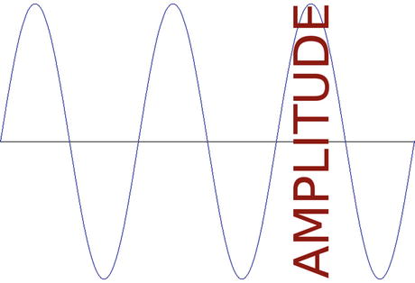
Figure 3-1.
Data resolution is specified using wave amplitude
Digital audio sample resolutions are defined with 8-bit, 12-bit, 16-bit, 24-bit, or 32-bit data. In digital imaging and digital video, data resolution is quantified by the number of 8-bit color channels; in digital audio, the resolution is quantified by the number of bytes of data used to define each of the audio samples being taken. Audacity samples at 32-bit data resolution, because you want to start high
and then optimize digital audio to one of the mainstream lower resolutions (as you’ll see in Chapter 12, where digital audio data footprint optimization is discussed).
Except for the 12-bit resolution for digital audio, which is actually rarely used, the 8-bit, 16-bit, 24-bit, and 32-bit data packet resolutions match up identically between digital imagery editing and digital audio editing. The most commonly used audio data resolutions are 8 bits in low-quality sound effects or voice tracks, 16 bits in music, and 24 bits in HD audio (again, music).
As with digital images, where more color yields a better image quality, in digital audio, a higher sample resolution always yields a better sound wave reproduction.
Thus, higher sampling resolutions, or using more data to reproduce a given sound wave sample, yields a higher audio playback quality at the expense of a larger data footprint.
This is the reason why 16-bit audio, termed “CD quality” audio, sounds better than 8-bit audio; just like true color JPEG or PNG24 imagery should always look better than 8-bit GIF indexed color images. Having a 12-bit digital audio resolution is a valuable option for getting higher quality vocal tracks or sound effects without having to use 16-bit or 24-bit data, because these audio data resolutions are more appropriate for high-quality music experiences or for the audio track in a film or digital video p
roduction.
In digital audio broadcasting, there’s a trend in using a 24-bit digital audio sampling resolution, known as “HD audio” in the consumer electronics industry.
HD digital audio broadcast radio and satellite radio now use a 24-bit data sampling resolution, so each audio sample, or slice of a sound wave, contains 16,777,216 (this is 24 bits in decimal) potential sample-resolution numeric accuracy.
Some of the newer iOS, Android, and Blackberry devices now support HD audio, starting with the smartphone products that are advertised as featuring HD-quality digital audio playback hardware (a 24-bit capable audio data decoding hardware chip). In order for a hardware device to play the HD audio format, you must have 24-bit audio hardware. I recommend using the 16-bit audio for the widest playback compatibility.
Data Sample Frequency: Data Samples per Second
Besides a digital audio sample resolution, you also have a digital audio
sampling frequency
.
This defines the number of data samples, at any given sample resolution, which are taken during one second of sample time. In digital imagery, sampling frequency is analogous to the number of pixels that are contained in a digital image. Sampling frequency is sometimes termed a sampling rate. You are familiar with the term CD quality audio, which is defined as using a 16-bit sample resolution and a 44.1 kHz sampling rate. This is taking 44,100 samples, each of which contains 16 bits of sample resolution, or the potential maximum 65,536 data values, for digital audio data held in each sample.
The sampling frequency is taken along the other (x) axis of the sound wave, or waveform, than the resolution is, so that each sample can also have a resolution.
The sampling rate is the number of resolution data samples in a full second of audio data along the frequency dimension of a digital audio waveform, as illustrated in Figure 3-2.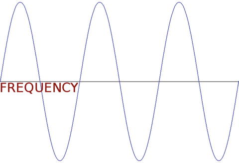
Figure 3-2.
The number of data samples are taken over the frequency
Common audio sample rates for the digital audio industry include 8 kHz, 11.25 kHz, 22.5 kHz, 32 kHz, 44.1 kHz, 48 kHz, 96 kHz, 192k Hz, and recently, 384 kHz. As you may have noticed, I like to use the ones that are evenly divisible by a power of two (8-bit), and so I gravitate toward 8 kHz (low quality), 32 kHz (medium quality), and 48 kHz (high quality).
Lower sampling rates, such as 8 kHz or 11.25 kHz, should be optimal for sampling “voice-based” digital audio, as well as sound effects, such as game sound effects, dialog tracks, or an audio e-book narration track, for example.
Medium-quality audio sample rates, such as 22.5 kHz or 32 kHz, are more appropriate in background music loops in games and some sound effects, such as rumbling thunder, which absolutely needs to have a high dynamic range to ensure higher fidelity digital audio reproduction. The same goes for using 22.5 kHz on vocal tracks in
high-quality vocals.
Higher audio sample rates, such as 44 kHz or 48 kHz, are more appropriate for music, which usually requires your highest fidelity reproduction.
Some sound effects, or even music, can get away with using lower 22.5 kHz or 32 kHz sampling rates, as long as the sampling resolution used is 16-bit quality or higher.
Ultimately, you have to use your ears as your guide during the digital audio optimization process, which you’ll do in Chapter 12 after you create and edit a data sample and need to ascertain what your “aural quality–to–digital audio asset file size” trade-off is going to be.
Data Sample Mathematics: Amount of Binary Data
Let’s do
some math to find out the number of bits of data that might be held in one second of raw (uncompressed) digital audio data. This is calculated by multiplying the sample resolution by the sampling frequency. A 16-bit sample resolution contains 65,536 potential data samples, and the sampling frequency is 44,100 samples per second. Multiplying these yields 2,890,137,600 data values available to represent one second of CD quality audio.
Digital audio data codecs compress this down to an amazingly small file size. The initial raw data footprint size is the starting point for digital audio data footprint optimization. So if you can get adequate quality using a lower sample resolution and (or) a lower sampling rate, the digital audio compression algorithm (codec) is able to do a much better job of exporting a more compact data file; that is, a smaller digital audio file size.
The same trade-off you have with a digital imaging asset exists with digital audio. If you include more data, you get a high-quality result at the cost of a larger file size. Audio codecs do a great encoding job. Fortunately, digital audio has better quality-to–file size results than digital imagery.
Sample Products: Sampler Hardware and Libraries
Although this book includes the work process for creating your own digital audio data samples, you can also obtain third-party, professional digital audio data samples in a number of different formats, including sampler keyboards and rack-mount hardware, sampler software, and sample libraries, which come on CD-ROM, DVD-ROM, or EPROM chips that install in the keyboard or rack-mount sampler hardware. If you want to be a composer, this is the best option because the instrument samples are done for you, so you can focus on creating musical compositions.
The most expensive sampling hardware is keyboard samplers, because they have a MIDI controller and a sample playback hardware architecture in one completely integrated instrument. Rack-mount sampler hardware is significantly less expensive, because it only has the sampler playback hardware and few moving parts other than some knobs, dials, sliders, and LCD readouts.
The next step down in expense is sample playback software. You need a MIDI controller to use it. This is the next most expensive option because it uses the computer processor as sample processing hardware to play the samples. With this solution, sample data comes on a CD-ROM or DVD-ROM, and is loaded onto the hard disk and played back by the sampler software using a MIDI controller after the instrument samples are loaded into the system memory.
Recording Digital Audio: Using Audacity
Since this is the third chapter, let’s start the process of using Audacity to record a data sample and to see how Audacity
works. As you can see in Figure 3-3, Audacity’s audio recording levels are located at the top center of the screen, exactly where they should be. Click Click to Start Monitoring to learn the ambient sound levels that your microphone is recording in your room. Audio levels show you the amplitude of the sound waves that you are recording.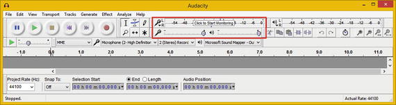
Figure 3-3.
Launch Audacity and click Click to Start Monitoring
You can see these levels (they animate, based on ambient noise) in Figure 3-4. I left Audacity at the default settings, because you will remove your ambient background noise in Chapter 6, which covers the Audacity noise removal algorithm and work process.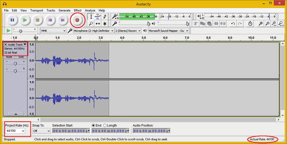
Figure 3-4.
Use the record button
to record your voice at 44.1 kHz
To the left of the digital audio level meters you see the
audio transport controls
. These include your standard play and pause buttons, as well as stop and record buttons. I’ve circled the record button, which you click and then say “digital audio editing fundamentals,” into your desktop microphone. I used a $9 Logitech stand microphone from Walmart on my workstation.
When you are finished recording, click the stop button to end the recording process. You see the sound waves shown in Figure 3-4 (or something similar) in the middle of the Audacity window.
As you can see in the bottom-right corner of Figure 3-4, Audacity shows you the actual sampling rate (sampling frequency) used in this waveform data (this is shown in the middle of the editing window). You can set the actual sampling rate before recording using the Project Rate (Hz) drop-down menu at the bottom-left corner. The sample rate and the sample resolution are shown on the left side of Figure 3-4; just as I said, the default Audacity sample settings are 32-bit resolution with a CD-quality 44.1 kHz sample frequency.
Now that you have the sample data that you’ll be refining over the next few chapters, let’s save your project, which you always want to do after creating any sample. This is done using the Audacity File ➤ Save Project menu sequence
, as shown in Figure 3-5.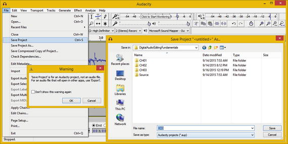
Figure 3-5.
Save you Audacity project using File ➤ Save Project
The first thing that you see is a Warning dialog that informs you that an AUP file format is not an audio (playback) file format, but instead an AUdacity Project data file format. This is shown on the left in Figure 3-5. Click the OK button, enter a File name for your Audacity project, and then click the Save button. I saved this sample as CH3.AUP in case you want to use it during Chapters 5–8.
Summary
In this chapter, you learned about digital audio data sampling concepts, techniques, and principles, as well as how to calculate sample data and how to record your own data samples using Audacity 2.1.1. You also learned about samplers and sample resolution along the y axis and sampling frequency along the x axis.
In the next chapter, you learn about digital audio data formats and digital audio data transmission principles.