Fault detection is the process of detecting failures, also known as faults, in a dynamical system. It is an important area for systems that are supposed to operate without human supervision. There are many ways of detecting failures. The simplest is using boolean logic to check against fixed thresholds. For example, you might check an automobile’s speed against a speed limit. Other methods include fuzzy logic, parameter estimation, expert systems, statistical analysis, and parity space methods. In this section, we will implement one type of fault detection system, a detection filter. This is based on linear filtering. The detection filter is a state estimator tuned to detect specific failures. We will design a detection filter system for an air turbine. We will also show how to build a graphical user interface (GUI) as a front end to the fault detection simulation.
10.1 Modeling an Air Turbine
Problem
We need to make a numerical model of an air turbine to demonstrate detection filters.
Solution
Write the equations of motion for an air turbine. We will use a linear model of the air turbine to simplify the detection filter design. This will allow us to model the system with a linear state space model.
How It Works
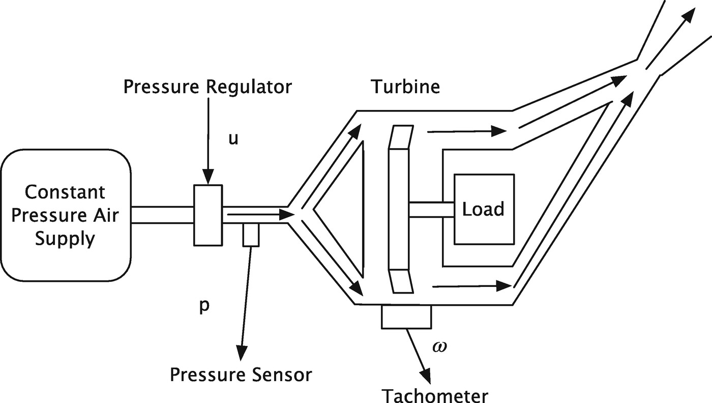
Air turbine. The arrows show the airflow. The air flows through the turbine blade tips causing it to turn.


The code for the right-hand side of the dynamical equations is shown in the following. Only one line of code is needed. The rest returns the default data structure. The simplicity of the model is due to its being a state space model. The number of states could be large, yet the code would not change.

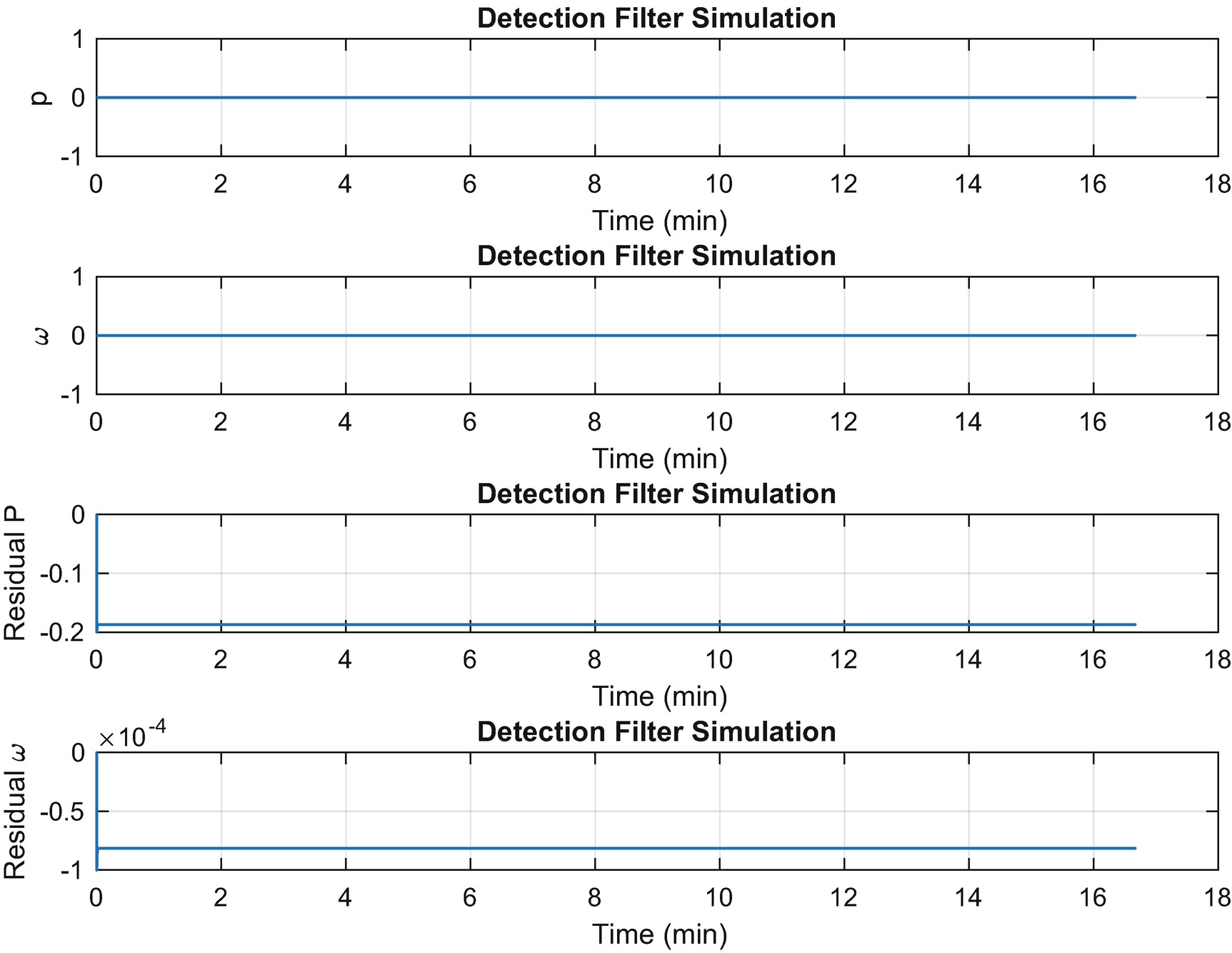
Air turbine response to a step pressure regulator input. The residuals are zero as expected.
10.2 Building a Detection Filter
Problem
We want to build a system to detect failures in our air turbine using the linear model developed in the previous recipe.
Solution
We will build a detection filter that detects pressure regulator failures and tachometer failures. Our plant model (continuous a, b, and c state space matrices) will be an input to the filter building function.
How It Works

 is the estimated pressure and
  is the estimated angular rate of the turbine. The D matrix is the matrix of detection filter gains. These feedback the residuals, the difference between the measured and estimated states, into the detection filter. The residual vector is
- 1.
The filter is stable.
- 2.
If the pressure regulator fails, the first residual
 is nonzero, but the second remains zero.
 - 3.
If the turbine fails, the second residual
 is nonzero, but the first remains zero.

The time constant τ 1 is the pressure residual time constant. The time constant τ 2 is the tachometer residual time constant. In effect, we cancel out the dynamics of the plant and replace them with decoupled detection filter dynamics. These time constants should be shorter than the time constants in the dynamical model so that we detect failures quickly. However, they need to be at least twice as long as the sampling period to prevent numerical instabilities.
We will write a function with three actions, an initialize case, an update case, and a reset case. varargin is used to allow the three cases to have different input lists. The function signature is
![]()
The header and syntax for DetectionFilter are shown as follows. We used LaTeX equations to describe the function.
The filter is built and initialized in the following code in DetectionFilter. The continuous state space model of the plant, in this case, our linear air turbine model, is an input. The selected time constants τ are also an input, and they are added to the plant model as in Equation 10.8. The function discretizes the plant a and b matrices and the computed detection filter gain matrix d.
![]()
The update for the detection filter is in the same function, as the next action in the switch statement. Note the equations implemented as described in the header.
Finally, we create a reset action to allow us to reset the residual and state values for the filter in between simulations. After this action, we end the switch statement.
10.3 Simulating the Fault Detection System
Problem
We want to simulate a failure in the plant and demonstrate the performance of the failure detection.
Solution
We will build a MATLAB script that designs the detection filter using the function from the previous recipe and then simulates it with a user selectable pressure regulator or tachometer failure. The failure can be total or partial.
How It Works
The script designs a detection filter using DetectionFilter from the previous recipe and implements it in a loop. Runge-Kutta integration propagates the continuous domain right-hand side of the air turbine, RHSAirTurbine. The detection filter is discrete time.
The script has two scale factors uF and tachF that multiply the regulator input and the tachometer output to simulate failures. Setting a scale factor to zero is a total failure, and setting it to one indicates that the device is working perfectly. If we fail one, we expect the associated residual to be nonzero and the other to stay at zero. Failures can be any number between zero and one. Partial failures are not necessarily related to a specific mechanical failure but are useful for testing the system.
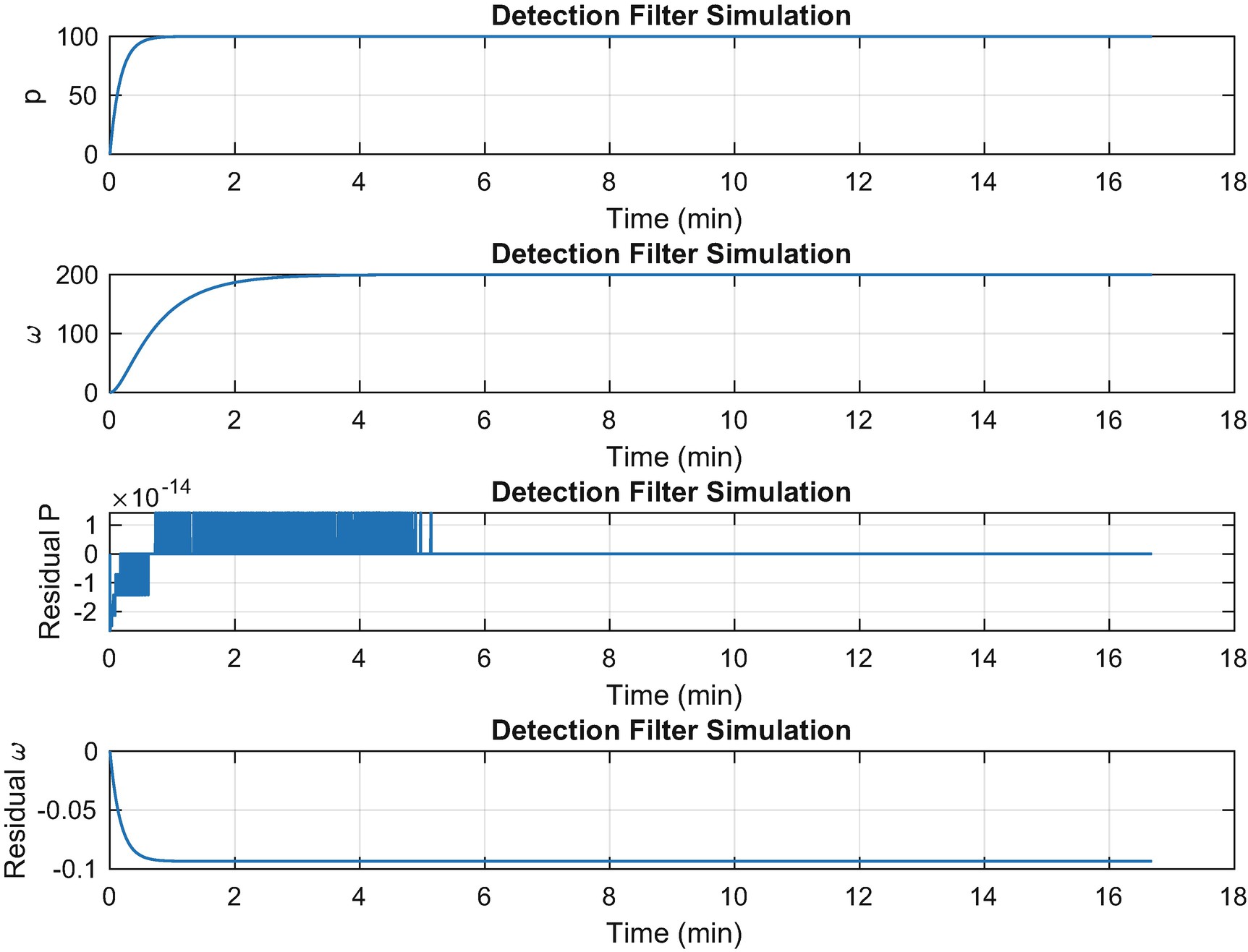
Air turbine response to a failed regulator.
Air turbine response to a failed tachometer.
10.4 Building a GUI for the Detection Filter Simulation
Problem
We want a GUI to provide a graphical interface to the fault detection simulation that will allow us to evaluate the filter’s performance.
Solution
- 1.
Set the residual time constants
- 2.
Set the end time for the simulation
- 3.
Set the pressure regulator input
- 4.
Introduce a pressure regulator or tachometer fault at any time
- 5.
Display the states and residuals in a plot
How It Works
Edit boxes for the simulation duration, residual time constants τ 1 and τ 2, pressure regulator setting u
Edit boxes for the pressure regulator and tachometer fault parameters, with buttons for sending the newly commanded values to the simulation
Text box for displaying the calculated detection filter gains
Run button for starting a simulation
Two plot axes
In order to change the fault parameters while the simulation is running, we will need the loop to be checking a variable that can be externally set by the GUI. We can do this using global variables.
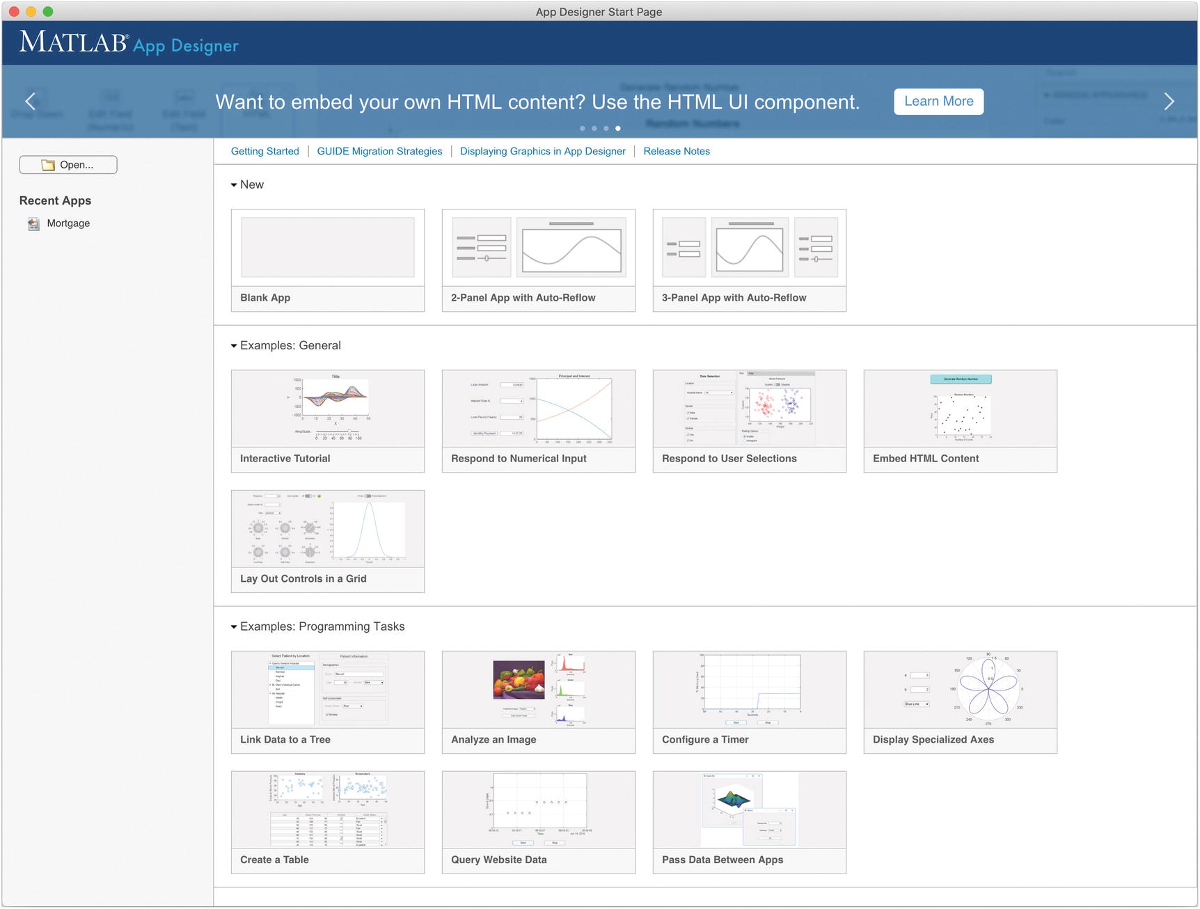
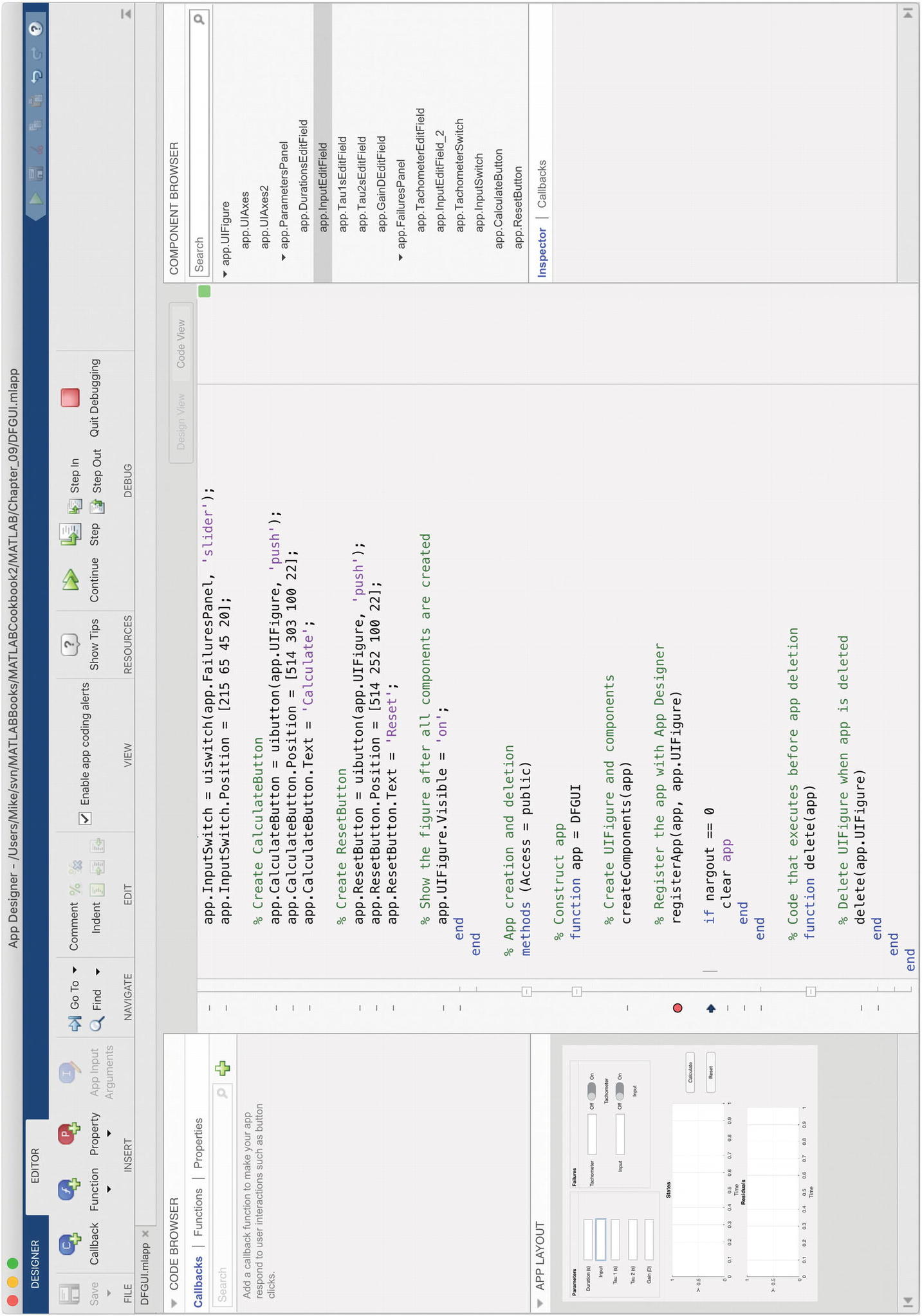
The interface to appdesigner.
Double-click the blank app template.
Add the app DFGUI. It will appear in your folder as DFGUI.mlapp.
Add the following to the blank template:
- 1.Parameter input boxes
- (a)
Duration
- (b)
Input
- (c)
Tau 1
- (d)
Tau 2
- (e)
Gains (2-by-2 matrix)
- 2.Failure input boxes
- (a)
Tachometer
- (b)
Input
- (c)
Send button for tachometer
- (d)
Send button for input
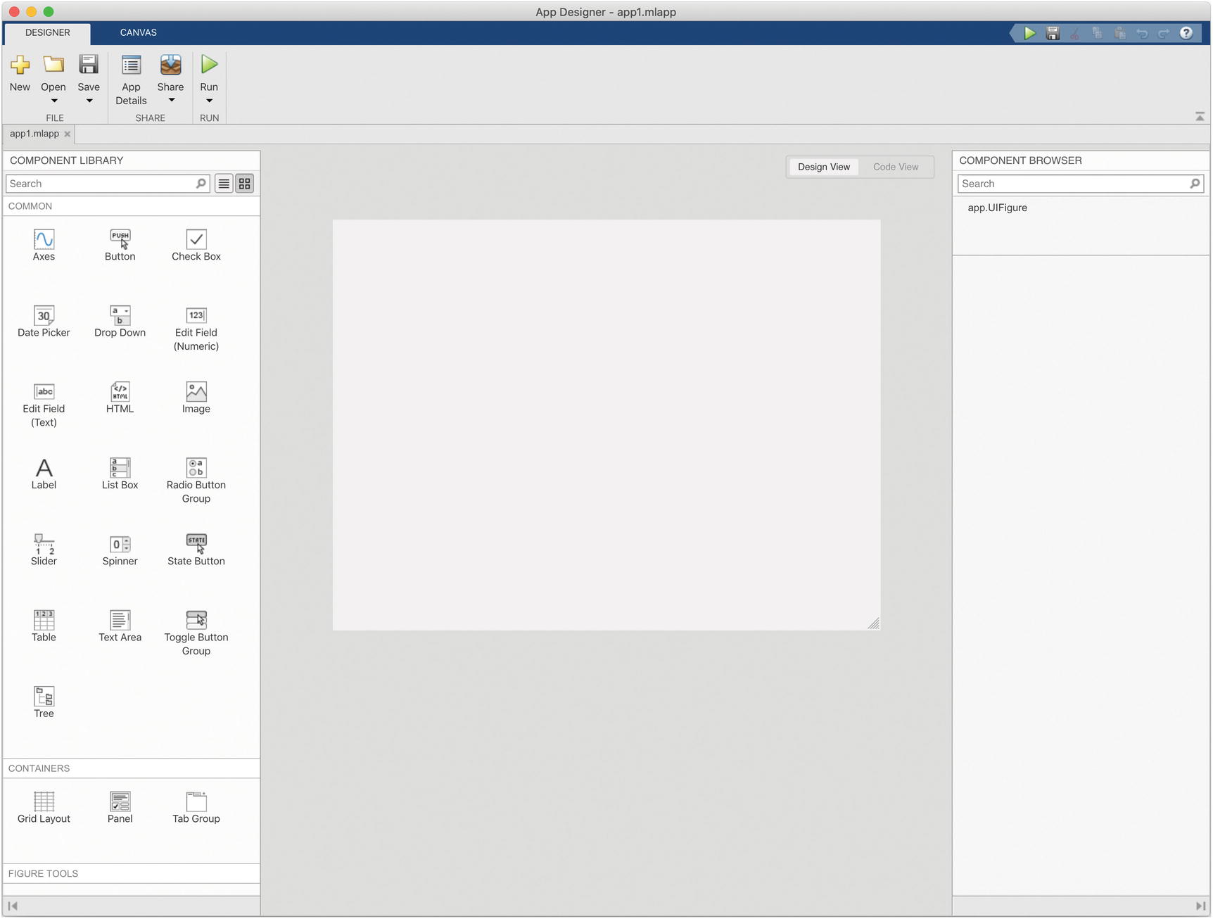 Figure 10.6
Snapshot of the blank app.
- 3.
Calculate button
- 4.
Reset button
- 5.
State plot
- 6.
Residual plot
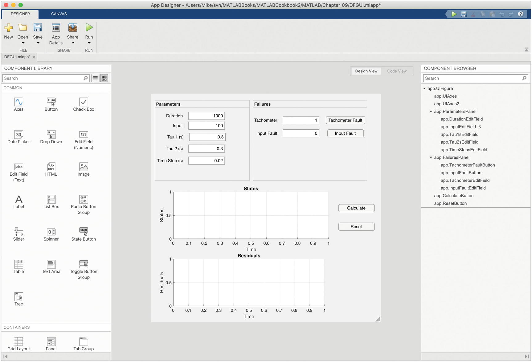
Snapshot of the app after the interface is done.
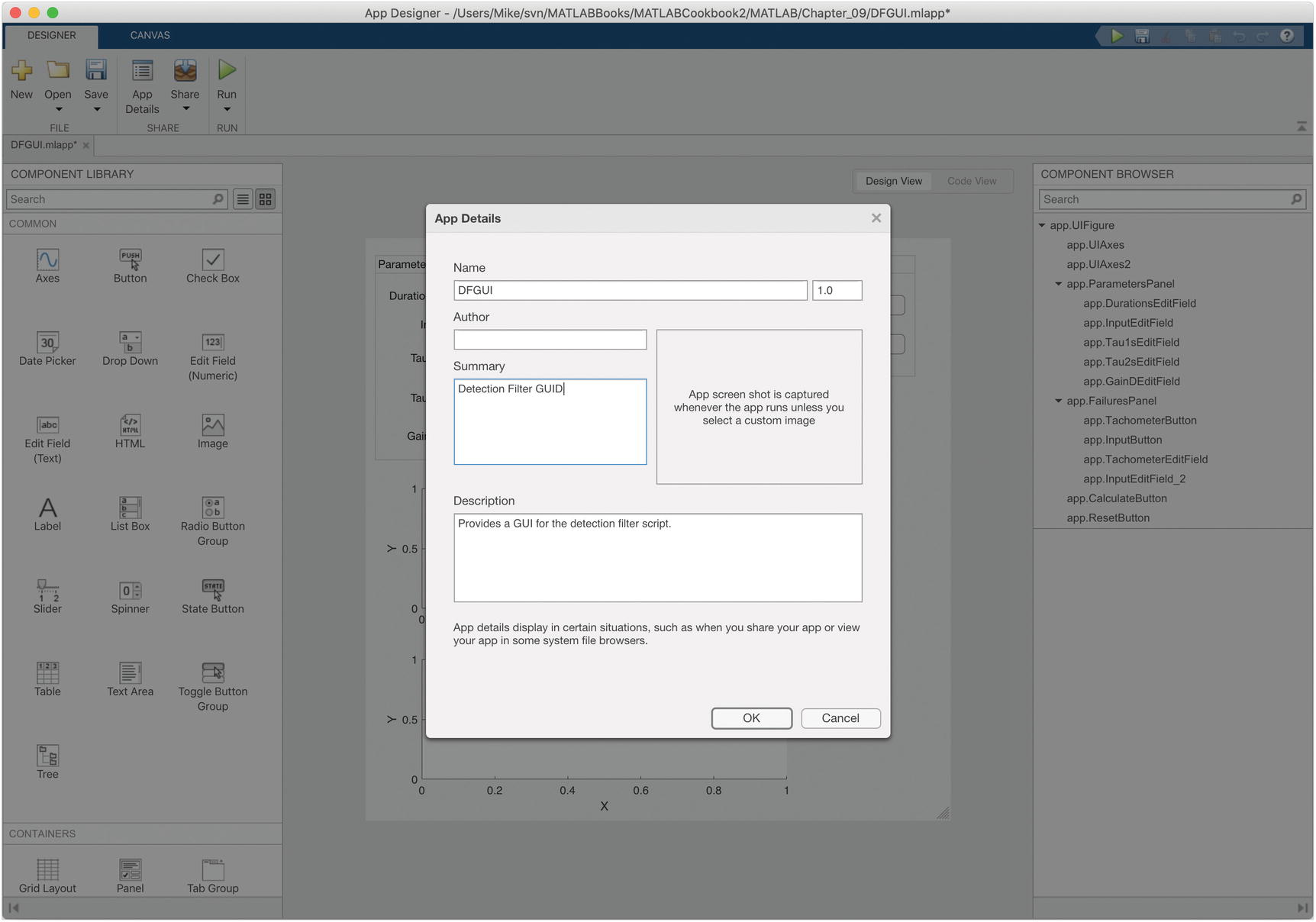
App Details let you add information about the app for users.

The app appears in the app menu. You get to this window by hitting the design app button.
We select the callback for calculate. The App Designer highlights where the code should go. We copy relevant code from the simulation script. We get the inputs from the text boxes.
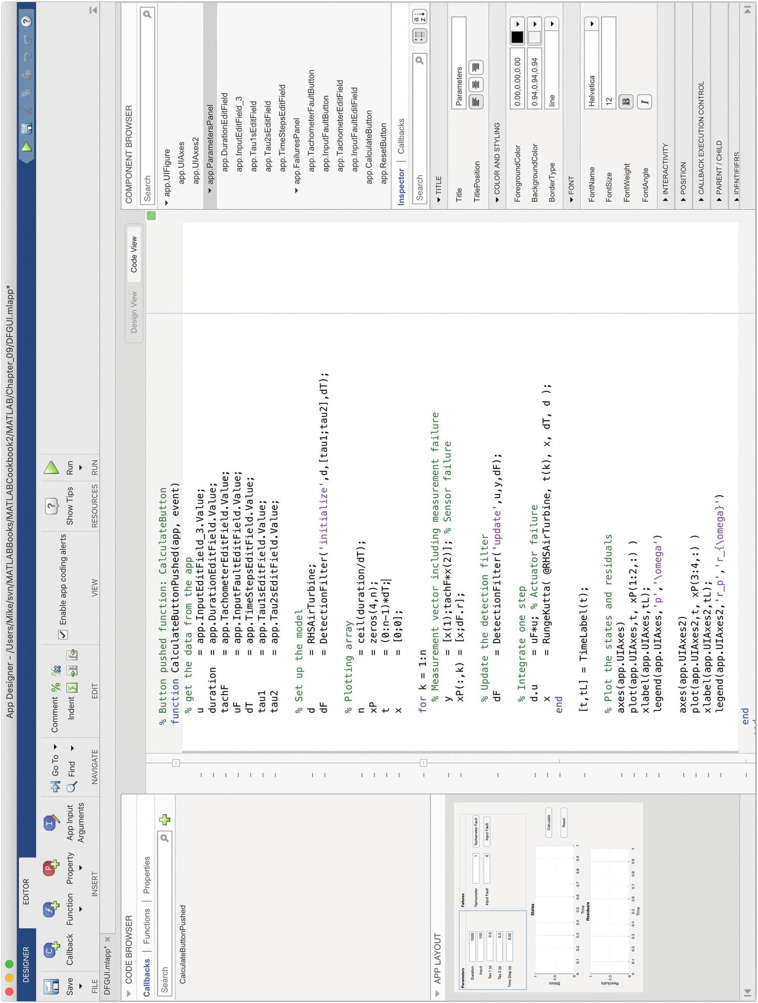
The light area is where the code goes. The code is from the simulation script.
You can use the debugger in the App Designer.
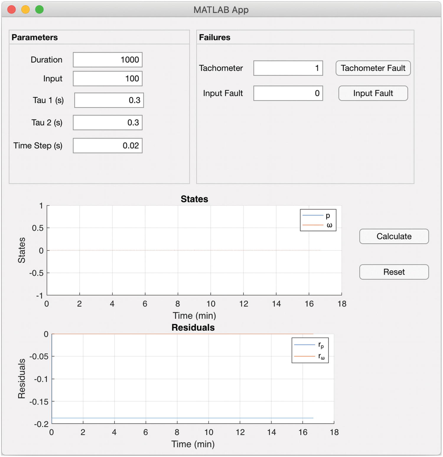
The app after a run.
Chapter Code Listing
File | Description |
RHSAirTurbine | Air turbine dynamical model in continuous state space form |
DetectionFilter | Builds and updates a linear detection filter |
DetectionFilterSim | Simulation of a detection filter |
DetectionFilterGUI | Run the detection filter simulation from a GUI |
DFGUI.m1App | App Designer app |
DFGUI.mlappinstall | DFGUI app installer |