Our aircraft model will be a three-dimensional point mass model. This models the translational dynamics in three dimensions. Translation is motion in the x, y, and z directions. An aircraft controls its motion by changing its orientation with respect to the wind (banking and angle of attack) and by changing the thrust its engine produces. In our model, we assume that our airplane can instantaneously change its orientation and thrust for control purposes. This simplifies our model but at the same time allows us to simulate most aircraft operations, such as takeoff, level flight, and landing. We also assume that the mass of the aircraft does not vary with time.
12.1 Creating a Dynamical Model of an Aircraft
Problem
We need a numerical model to simulate the three-dimensional trajectory of an aircraft in the atmosphere. The model should allow us to demonstrate control of the aircraft from takeoff to landing.
Solution
We will build a six-state model using flight path coordinates. Our controls will be the roll angle, angle of attack, and thrust. We will not simulate the attitude dynamics of the aircraft. The attitude dynamics are necessary if we want to simulate how long it takes for the aircraft to change the angle of attack and roll angle. In our model, we will assume the aircraft can instantaneously change the angle of attack, roll angle, and thrust.
How It Works

Flight path coordinates in two dimensions.


 is the drag at zero lift. k is the drag from the lift coupling coefficient. Polar comes from the
  term. This lift model is only valid for small angles of attack α as it does not account for stall, which is when the airflow becomes detached from the wing and the lift goes to zero rapidly.
Our RHS function that implements these equations is RHSAircraft. Notice that the equations are singular when v = 0 in Equation 12.2. We warn about this in the header. If called without arguments, the functions return the data structure. This is a handy way of making a complex function easier to use. It also gives the user an idea of what the parameters should be. All parameters must be in Meters-Kilogram-Second (MKS) units.

The function body is shown in the following. We assemble the state derivative, sDot, as one array since the terms are simple. Each element is on a separate line for readability. We return D and LStar as auxiliary outputs for use by the equilibrium calculation.


A more sophisticated right-hand side would pass function handles for the drag and lift calculations so that the user could use their own model. We pass a function handle for the atmospheric density calculation to allow the user to select their density function. We could have done the same for the aerodynamics model. This would make RHSAircraft more flexible.
Notice that we had to write an atmospheric density model, AtmosphericDensity, to provide as a default for the RHS function. This model uses an exponential equation for the density, which is the simplest possible representation. The function has a demo demonstrating the model which uses a log scale for the plot. This function also plots the results if no outputs are requested. This is also useful for helping users figure out what a function does.
12.2 Finding the Equilibrium Controls for an Aircraft Using Numerical Search
Problem
We want to find roll angles, thrusts, and angles of attack that cause the velocity, flight path angle, and bank angle state (roll angle) derivatives to be zero. This is a point of equilibrium. This is commonly called the trim condition.
Solution
We will use the Downhill Simplex algorithm, via the MATLAB function fminsearch, to find the equilibrium angles. fminsearch supports multivariable unconstrained optimization. The optimization toolbox in MATLAB provides additional functions with more options, such as handling constraints, that is, limits on the controls.
How It Works


The function, EquilibriumControl.m, uses fminsearch in a loop to handle multiple states. Within the loop, we compute an initial guess of the control. The thrust will need to balance the drag so we compute this at zero angle of attack. The lift must balance gravity so we compute the angle of attack from that relationship. Without a reasonable initial guess, the algorithm will converge to a local minimum but not necessarily the global minimum. The cost function is nested within the control function. The function can solve for multiple sets of states, hence the n.
![]()

The default output is to plot the results.

The cost sub (subfunction) function is shown in the following. We use a quadratic cost that is the unweighted sum of the squares of the state derivatives. The cost is the quantity that fminsearch tries to make as small as possible.
The function has a built-in demo that looks at the thrust and angle of attack at a constant velocity but increasing altitude, from 0 to 10 km. Built-in demos are always good, even if you are the only person who ever uses the function.
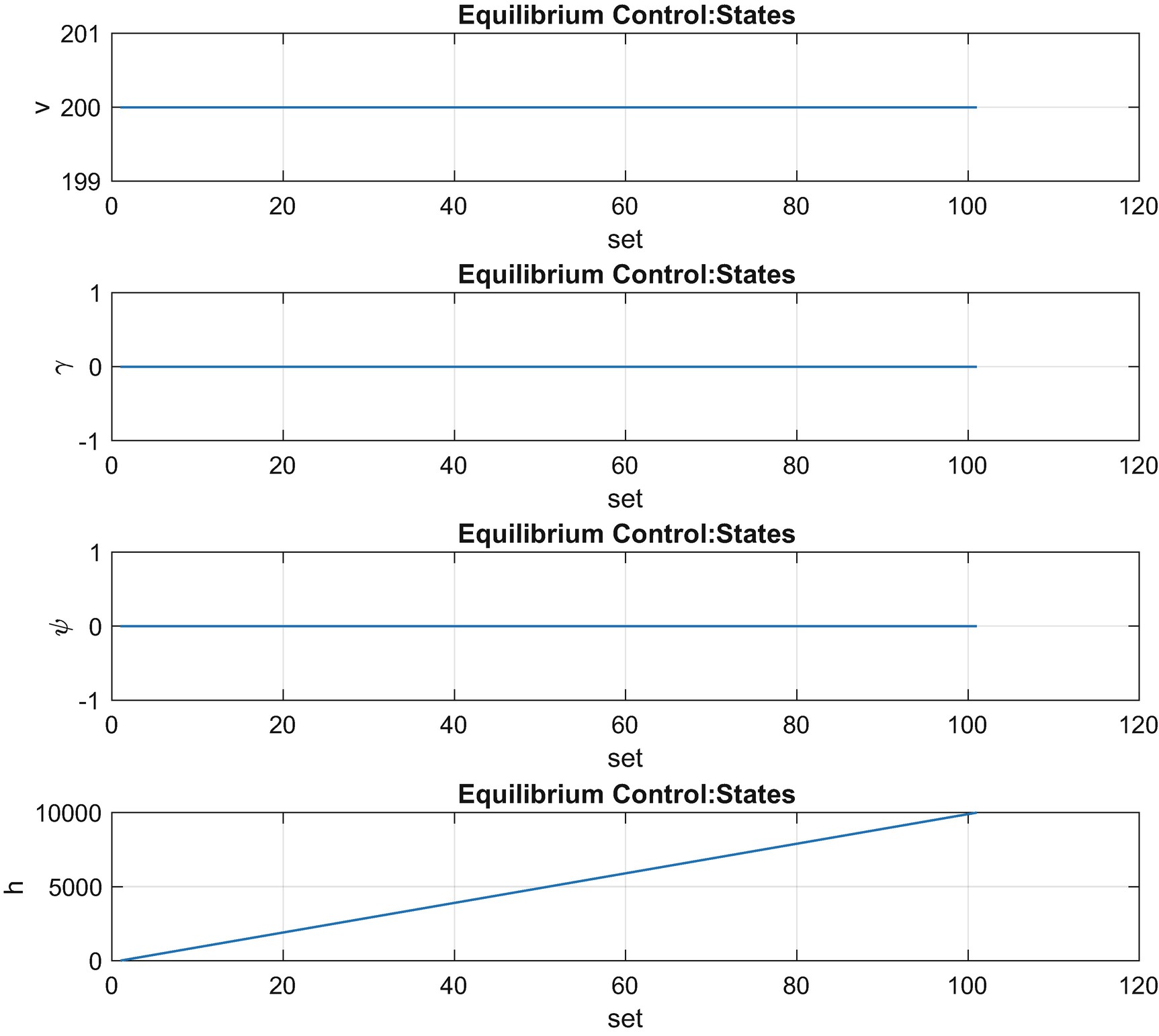
States for the demo. Only the altitude (h) is changing, following the desired flight path.
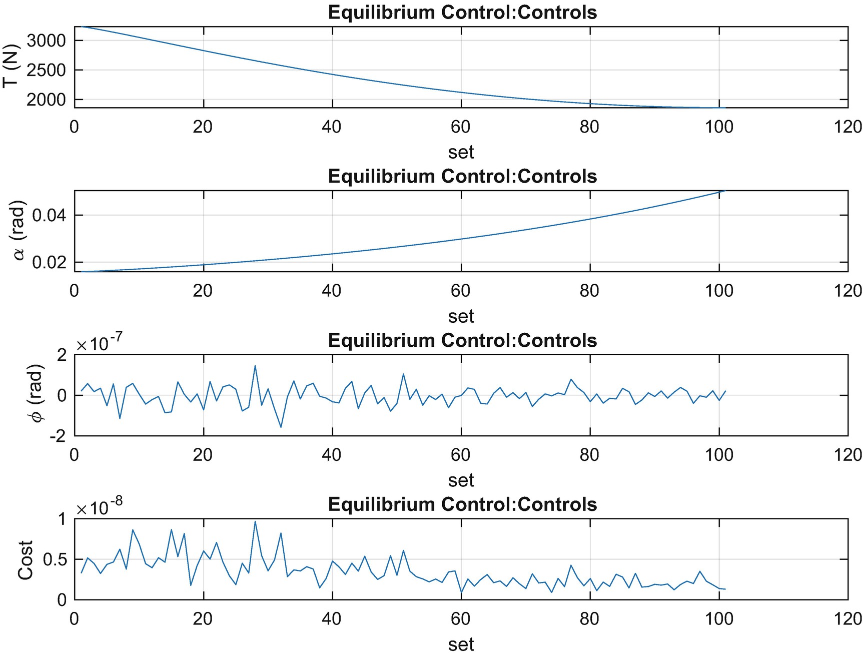
Controls for the demo. The thrust decreases with altitude and angle of attack increases.
In Figure 12.3, we also plot the cost. The cost should be nearly zero if the function is working as desired.
During debugging while writing a function requiring optimization, it may be helpful to have additional insight into the numerical search process. While we only need umin, consider the additional outputs available from fminsearch in this version of the function call.
![]()
The output structure will include the number of iterations, and the exit flag will indicate the exit condition of the function: whether the tolerance was reached (1), the maximum number of allowed iterations was exceeded (0), or if a user-supplied output function terminated the search (-1). We put a breakpoint in the script to check these outputs. For a state of v = 200 and h = 300 at k = 4, the output will be
So we can see that the search required 141 iterations and that the thrust increased to 3180.7 N from our initial guess of 2880.4 N. The resulting cost is 3 × 10⁻⁹. For more information, set the Display option of fminsearch to iter or final, with the default being notify. In this case, the options look like
![]()
and the following type of output will be printed to the command window:
For additional insight, we can add a plot function to be called at every iteration. MATLAB provides some default plot functions, for example, optimplotfval plots the cost function value at every iteration. You have to actually open optimplotfval in an editor to learn the necessary syntax. We add the function to the optimization options like this:
![]()

Function value plot using optimplotfval.
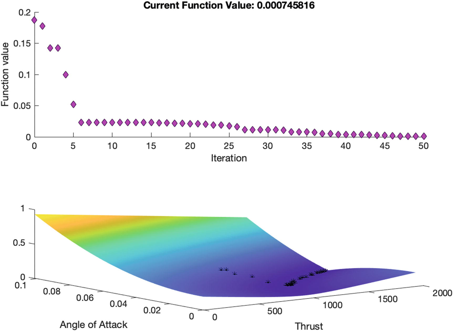
Custom optimization plot function using a surface.
![]()
We wrote two functions, one to generate the surface and a second to plot the iteration step. MATLAB sets the iteration value to zero during initialization, so in that case we generate the surface from the given initial state. For all other iteration values, we plot the cost on the surface using an asterisk.

Note, finally, that to see the default set of options MATLAB uses for fminsearch, call optimset with the name of the optimization function.
We see that the default tolerances are equal, at 0.0001, and the number of function evaluations and iterations is dependent on the number of variables in the input state x.
12.3 Designing a Control System for an Aircraft
Problem
We want to design a control system for an aircraft that will control the trajectory and allow for a three-dimensional motion.
Solution
We will use dynamic plant inversion to feedforward the desired controls for the aircraft. Proportional controllers will be used for thrust, angle of attack, and roll angle to adjust the nominal controls to account for disturbances such as wind gusts. We will not use feedback control of the roll angle to control the heading, ψ. This is left as an exercise for the reader.
How It Works

 is proportional to v. Our control variables are the roll angle ϕ, angle of attack α, and thrust T.


This is what happens when you perform a coordinated turn. Basically, this equation shows that in order to maintain the same level of responsiveness in longitudinal control (effective time constant of τ γ) during a turn (when ϕ is nonzero), the control gain on α must be increased. The bank angle during a turn causes a small reduction in the lift force for a given angle of attack. The flight path angle control is achieved by modulating α to vary the lift force. To maintain the same flight path angle response during a turn, we would have to maintain the same lift force through a corresponding increase in the angle of attack. We put the control system in the function AircraftControl.
The performance of the control system will be shown in the simulation recipe. The function requires information about the flight conditions including the atmospheric density. It first uses EquilibriumControl to find the controls that are needed when we are at the set point. The aircraft data structure is required. Additional inputs are the time constants for the controllers and the set points. We compute the atmospheric density in the function using feval and the input function handle. This should be the same computation as is done in RHSAircraft.
12.4 Plotting a 3D Trajectory for an Aircraft
Problem
We want to plot the trajectory of the aircraft in three dimensions and show the aircraft axes and times along the trajectory.
Solution
Demo of the aircraft trajectory function.
How It Works
We use plot3 to draw the 3D display. Our function Plot3DTrajectory.m allows for argument pairs via varargin.

We skip the demo code for now and show the drawing code next. There are similarities with our 2D plotting function, PlotSet. We use text to insert time labels and a patch object to draw the ground.
The plot commands are straightforward. If a time array is entered, it will draw the times along the track using sprintf and text. We use TimeLabel to get reasonable units. It will also draw the aircraft axes using the nested function DrawAxes.
This function draws an axis system for the aircraft, x out the nose, y out the right wing, and z down. It uses the state vector so it needs to convert from γ and ψ to rotation matrices. The axis system is in wind axes.
The function takes parameter pairs to allow the user to customize the plot. The parameter pairs are processed here just after the defaults are set:
We use lower in the switch statement to allow the user to input capital letters and not have to worry about case issues. Most of the parameters are straightforward. The time input could have been done in many ways. We chose to allow the user to enter specific times for the time labels. As part of this, the user must enter the indices to the state vector.
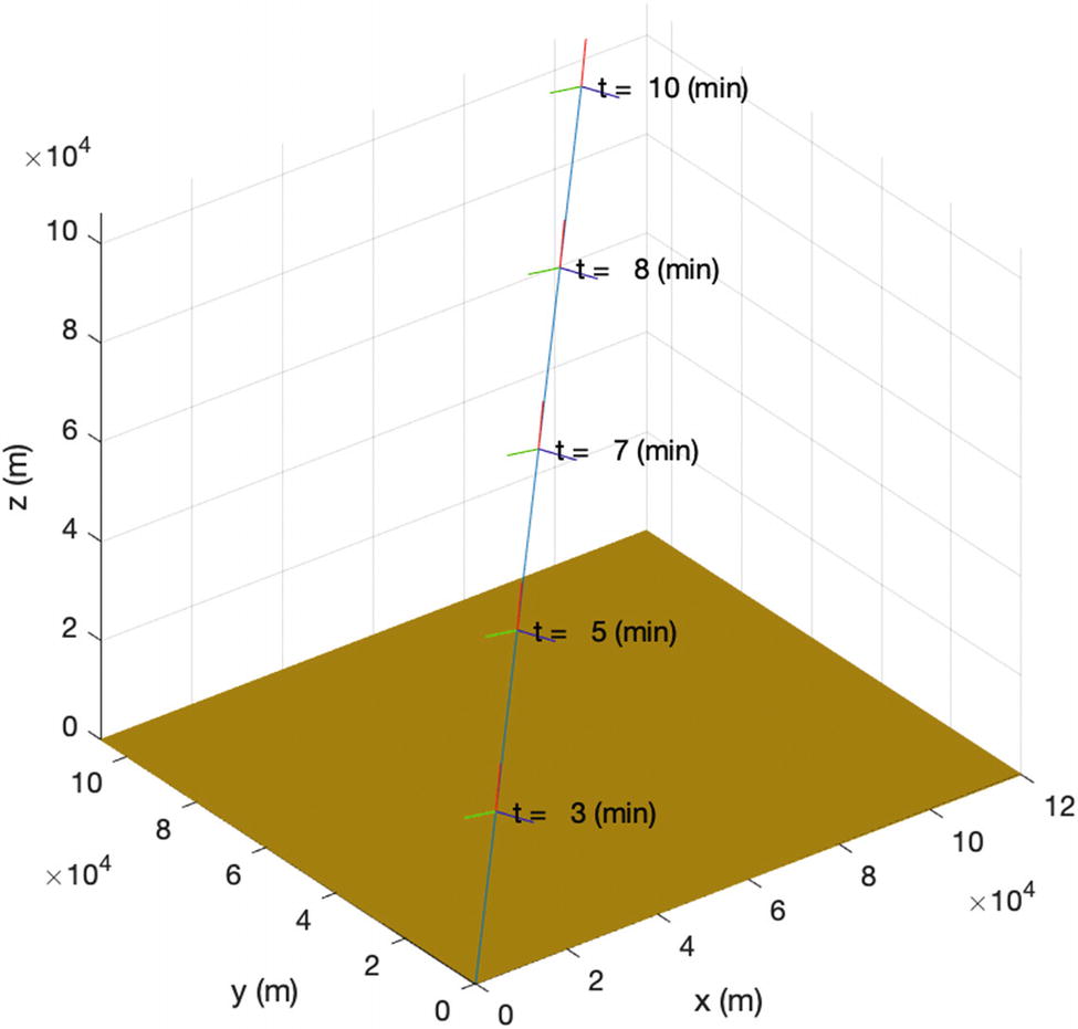
The function includes a demo. You can type Plot3DTrajectory and get the example trajectory shown in Figure 12.6. In the case of a graphics function, the demo literally shows the user what the graphics should look like and provides examples about how to use the function.
12.5 Simulating the Controlled Aircraft
Problem
We want to simulate the motion of the aircraft with the trajectory controls.
Solution
We will create a script with the control system and flight dynamics. The dynamics will be propagated by RungeKutta. This is a fourth-order method, meaning the truncation errors go as the fourth power of the time step. Given the typical sample time for a flight control system, the fourth order is sufficiently accurate for flight simulations. We will display the results using our 3D plotting function Plot3DTrajectory described in the previous recipe.
How It Works
The simulation script reads the data structure from RHSAircraft and changes values to match an F-35 fighter. The model only involves the thrust and drag, and even these are very simple models. The initial flight path angle and velocity are set. We turn on the control and establish the set points and time constants for the velocity and flight path angle states. For the output, we plot the states, control, and a 3D trajectory.

The script begins with obtaining our default data structure from the RHS function.
If the control is off, we set the thrust and angle of attack to constant values to balance the drag and gravity. The set points for velocity and flight path angle are slightly different than the initial conditions. This will allow us to demonstrate the transient response of the controller.
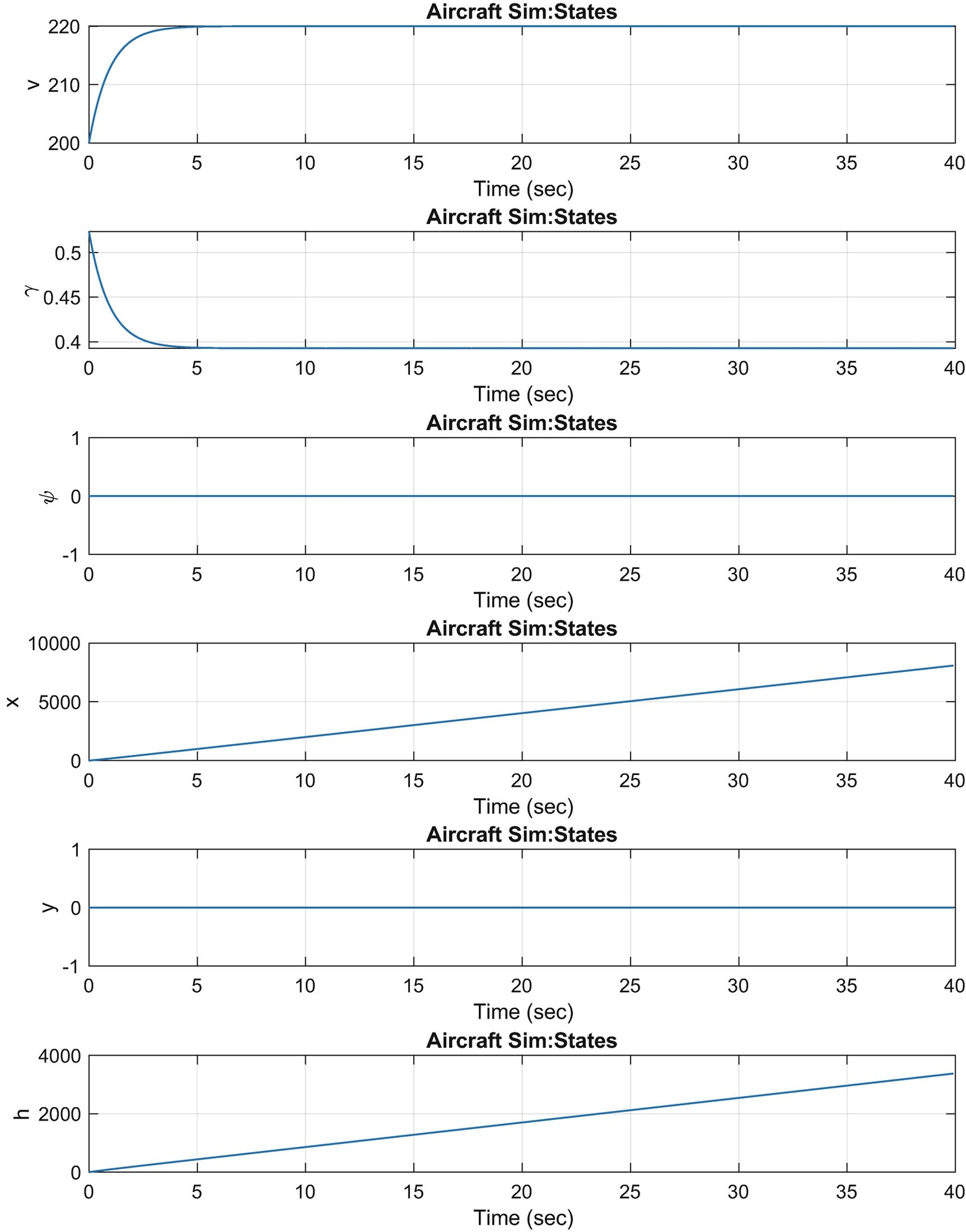
Velocity and flight path angle converge to their desired values.

The controls converge to the steady-state values and then change slowly to accommodate the decrease in atmospheric density as the aircraft climbs.
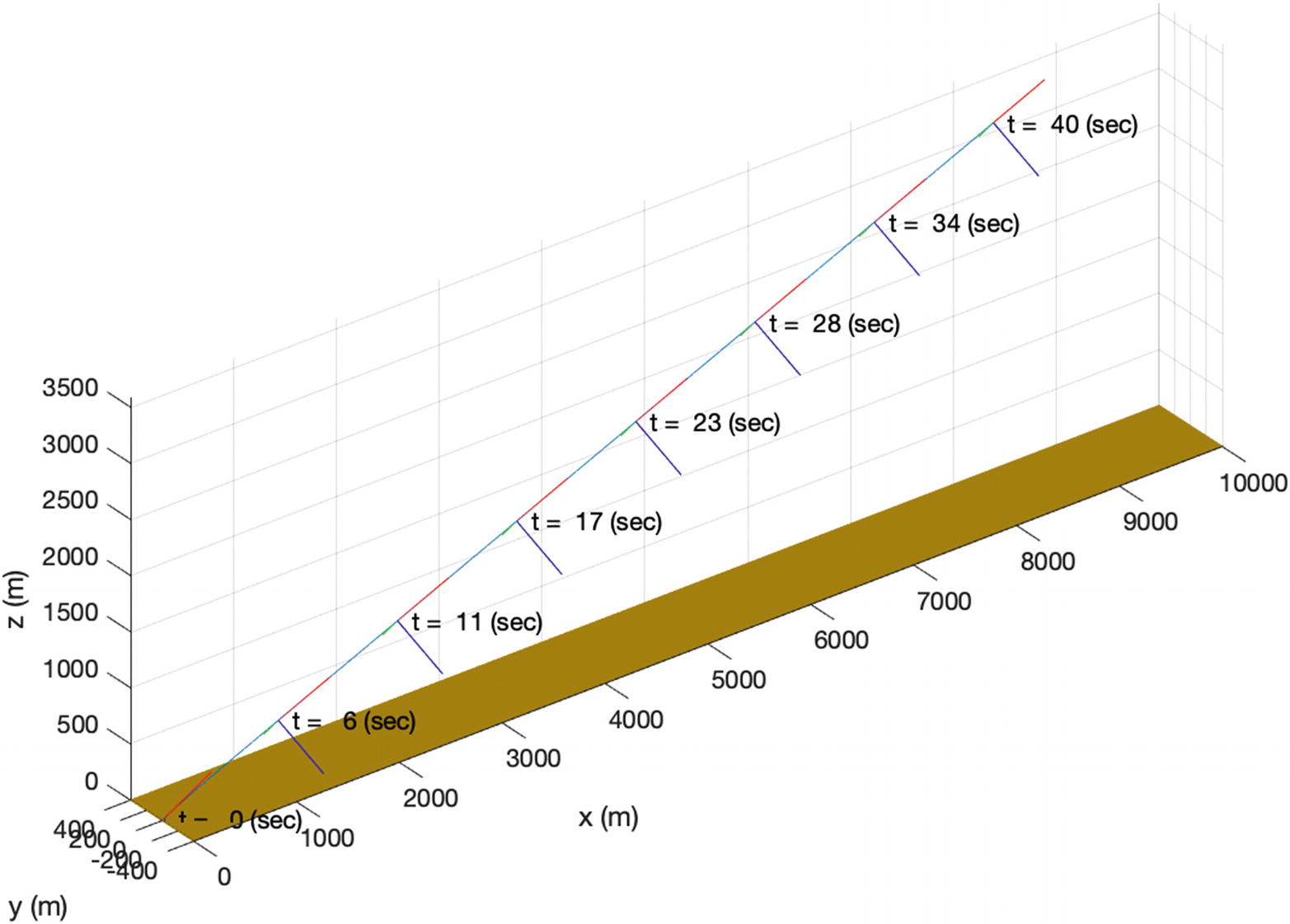
The aircraft trajectory.
This simulation assumes perfect state feedback, without noise. If there were noise or errors in the model parameters, we would see more control activity. Noise filtering, and possibly more complex controllers, might be required.
12.6 Draw an Aircraft
Problem
We want to visualize the orientation of an aircraft in three dimensions.
Solution
We will write a MATLAB visualization tool that will show an aircraft in three dimensions. The model will be from a Wavefront OBJ file.
How It Works
There are many visualization formats. One of the easiest to use is the Wavefront OBJ format. This is a text file with lines representing vertices, faces, surface normals, and texture coordinates. We will only use the faces and vertices. Some lines from the Gulfstream.obj file are shown in the following. v means vertex; f means face. There are only three vertices per face. OBJ can handle faces with any number of vertices, but graphics engines are more efficient when all of the polygons are triangles. mtllib gives the name of the material library that will be used to get textures and colors for the surfaces. g and o break the file into components. No hierarchy information is given in the file. If you want to articulate the object, you need to get the information from another source. For example, for the vertices, give its absolute position in the aircraft. If you wanted to rotate it, you would need to know its axis of rotation and its location in the body. You can see how this is done later in the code where we draw the meshes.
usemtl says use the particular material in the material library file. The slashes in the faces denote the vertex number/texture number and normal number. The vertices are numbered from 1 to n in the file. We don’t use the material library in our code.
The function LoadOBJ loads an OBJ file and breaks it into components using the g lines. From the preceding example, you can see that one component will be AileronL.
The function DrawAircraft creates a 3D view of the aircraft and animates it.
The main loop is a switch function. Actions are “initialize,” “update,” “movie,” and “close.” The “initialize” action sets up the axes.

The code in DrawMesh draws the vertices and faces for the component m. The only parts of the components used are the vertices and faces. The Phong lighting is a type of OpenGL lighting that approximates real lighting. Notice that the edge lighting can be different from the face lighting.
The following code updates the patches for the aircraft. It also updates the time uicontrol. It gets the vertices for each component, rotates the vertices, and then translates them. The GUI automatically changes the limits so that the plane remains centered. You will see, when you run the demo, the axis numbers change as the aircraft moves. We also call the function DrawAlphaBeta to draw axes and annotate them. getframe gets the information in the frame for use in a movie.


The following code runs the demo. We need to generate the position, velocity, and orientation. The orientation is defined by an attitude or orientation quaternion. Euler angles are another possibility, but they are computationally slower than quaternions. A quaternion can be thought of as an axis of rotation and an angle about that axis. The four elements are not independent since the sum of the squares of the elements of a quaternion equals 1. Quaternions are used in computer graphics and for spacecraft. A quaternion can be replaced by a transformation matrix. However, the latter is harder to handle since it is 3-by-3, while the quaternion is a 4-by-1 array. It is simpler to store a set of “n” 4-by-1 quaternions (e.g., as a 4-by-n matrix) than it is to store a set of “n” 3-by-3 rotation matrices.
The demo loads the aircraft and then calls the movie action in DrawAircraft. This returns a pointer to a movie frame that can later be saved. If you don’t want a movie, call DrawAircraft with “update.” The rotation of the aircraft is the product of two matrices. One is a constant pitch (rotation about Y) matrix and the other a time-varying roll (rotate about X) matrix. You can create arbitrary rotation matrices by multiplying multiple rotation matrices together.
We create an array consisting of the column matrix [1;0;-0.2] by dot multiplication with a row array of ones. This is a relatively new MATLAB feature. MATLAB figures out that you want 100 copies of the column array.
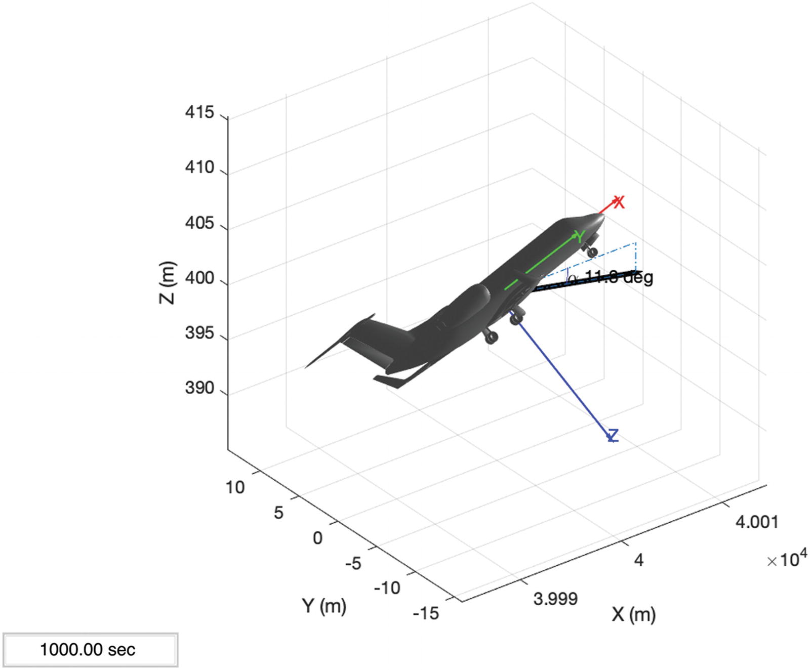
The aircraft at the end of the demo.
Chapter Code Listing
File | Description |
|---|---|
DrawAircraft | Draw a 3D model of an aircraft |
RHSAircraft | Six degrees of freedom RHS for a point mass aircraft |
AtmosphericDensity | Atmospheric density as a function of altitude from an exponential model |
EquilibriumControl | Find the equilibrium control for a point mass aircraft |
AircraftControl | Compute the angle of attack and thrust for a 3D point mass aircraft |
Plot3DTrajectory | Plot a 3D trajectory of an aircraft with times and local axes |
AircraftSim | A trajectory control simulation of an aircraft |