The SCARA robot (Selective Compliance Articulated Robot Arm) is a simple industrial robot that can be used for placing components in a two-dimensional space. We will derive the equations of motion for a SCARA robot arm. It has two rotational joints and one prismatic joint. A prismatic joint allows only linear motion. Each joint has a single degree of freedom. A SCARA robot is broadly applicable to work where a part needs to be inserted in a two-dimensional space or where drilling needs to be done.
Our input to the robot system will be a new location for the arm effector. We have to solve two control problems. One is to determine what joint angles we need to place the arm at a particular xy coordinate. This is the inverse kinematics problem. The second is to control the two joints so that we get a smooth response to commands to move the arm. We will also develop a custom visualization function that can be used to create animations of the robot motion.
For more information on the dynamics used in this chapter, see Example 9.8.2 (p. 405) in Lung-Wen Tsai’s book Robot Analysis: The Mechanics of Serial and Parallel Manipulators, John Wiley & Sons, New York, 1999.
8.1 Creating a Dynamical Model of the SCARA Robot
Problem
The robot has two rotational joints and one prismatic or linear “joint.” We need to write the dynamics that link the forces and torques applied to the arm to its motion so that we can simulate the arm.
Solution
The equations of motion are derived using the Lagrangian formulation. We will need to solve a set of coupled linear equations in MATLAB.
How It Works
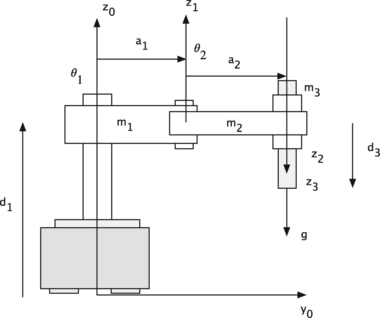
SCARA robot. The two arms move in a plane. The plunger moves perpendicular to the plane.


Note that in developing this inertia matrix, the author is treating the links as point masses and not solid bodies.
The inertia matrix is symmetric as it should be. There is coupling between the two rotational degrees of freedom but no coupling between the plunger and the rotational hinges. The inertia matrix is not constant, so it cannot be precomputed.
First, we will define a data structure for the robot, in SCARADataStructure.m, defining the length and mass of the links, and with fields for the forces and torques that can be applied. The function can supply a default structure to be filled in, or the fields can be specified a priori.
Then we write the right-hand-side (RHS) function from our equations. We need to solve for the state derivatives  which we will do with a left matrix divide. This is easily done in MATLAB with a backslash, which uses a QR, triangular, LDL, Cholesky, Hessenberg, or LU solver, as appropriate for the inputs. The function does not have a built-in demo as this impacts performance in RHS functions, which are called repeatedly by integrators. Note the definition of the constant for gravity at the top of the file. The inertia matrix is returned as an additional output. This is handy for debugging.
8.2 Customize a Visualization Function for the Robot
Problem
We would like to be able to visualize the motion of the robot arm, without relying on simple time histories or 3D lines.
Solution
We will write a function to draw a 3D SCARA robot arm. This will allow us to easily visualize the movement of the robot arm.
How It Works
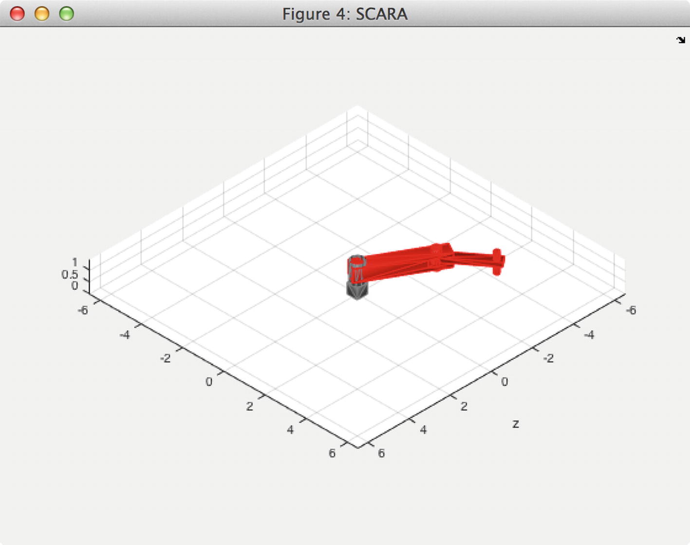
SCARA robot visualization using patch.
This function’s first argument is an action. We define an initialization action to generate all the patch objects, which are stored in a persistent variable. Then, during the update action, we only need to update the patch vertices. The function has one output, which is movie frames from the animation. Note that the input x is vectorized, meaning we can pass a set of states to the function and not just one at a time. The header of the function is as follows.
“patch” is a computer graphics term for a part of a surface. It consists of vertices organized into faces.
Next, we show the body of the main function. Note that the function has a built-in demo demonstrating a vector input with 100 states. The function will initialize itself with default data if the data structure d is omitted.

Note that we used subfunctions for the Initialize and Update actions. This keeps the switch statement clean and easy to read. In the Initialize function, we define additional parameters for creating the box and cylinder objects we use to visualize the entire robot arm. Then we use patch to create the graphics objects, using parameter pairs instead of the (x, y, z) input. Specifying the unique vertices this way can reduce the size of the data needed to define the patch and is simple conceptually. See the Introduction to Patch Objects and Specifying Patch Object Shapes sections of the MATLAB help for more information. The handles are stored in the persistent variable p. We only show the creation of the base. The patch function creates the 3D object from vertices and faces. Phong lighting is defined.

The Update function updates the vertices for each patch object. The nominal vertices are stored in the persistent variable p and are rotated using a transformation matrix calculated from the sine and cosine of the link angles. If there is an output argument, the function uses getframe to grab the figure as a movie frame.
The subfunctions Box, Cylinder, and UChannel create the vertices and faces for each type of 3D object. Faces are defined using indices of the vertices, in this case, triangles. We will show the Box function here to demonstrate how the vertices and faces matrices are created.
8.3 Using Numerical Search for Robot Inverse Kinematics
Problem
The goal of the robot controller is to place the end effector at a desired position. We need to know the link states corresponding to this position.
Solution
We will use a numerical solver to compute the robot states. The MATLAB solver is fminsearch, which implements a Nelder-Mead minimizer.
Nelder-Mead is also known as downhill simplex. This is not to be confused with the simplex algorithm.
How It Works
![$$left [x;y;z
ight ]$$](https://imgdetail.ebookreading.net/202109/5/9781484261248/9781484261248__9781484261248__files__images__335353_2_En_8_Chapter__335353_2_En_8_Chapter_TeX_IEq2.png) . z is determined by d
1 − d
3 from Figure 8.1 in Recipe 8.1. x and y are found from the two angles a
1 and a
2. The position vector for the arm end effector is
. z is determined by d
1 − d
3 from Figure 8.1 in Recipe 8.1. x and y are found from the two angles a
1 and a
2. The position vector for the arm end effector is 
We will use this equation for the position to create a cost function that can be passed to fminsearch. This will compute the state which results in the desired position. The resulting function demonstrates a nested cost function, a built-in demo, and a default plot output. Note that we use a data structure as returned by optimset to pass parameters to fminsearch.
The function creates a video using a VideoWriter object and the frame data returned by DrawSCARA. Before VideoWriter was introduced, this could be done with movie2avi.
8.4 Developing a Control System for the Robot
Problem
Robot arm control is a critical technology in robotics. We need to be able to smoothly and reliably change the location of the end effector. The speed of the control will determine how many operations we can do in a given amount of time, thus determining the productivity of the robot.
Solution
We will solve this problem using the inverse kinematics function discussed earlier and then feeding the desired angles into two PD controllers as developed in the Chapter 7.
How It Works

The first step is to specify a desired position for the end effector and use the inverse kinematics function to compute the target states corresponding to this location.
Next is the code that designs the controllers, one for each joint, using PDControl. Note that we use identical parameters for both controllers. We set the damping ratio, zeta, to 1.0 to avoid overshoot. Recall that wN, the undamped natural frequency, is the bandwidth of the controller; the higher this frequency, the faster the response. wD, the derivative term filter cutoff, is set to 5–10 times wN so that the filter doesn’t cause lag below wN. The dT variable is the time step of the simulation.
This is the portion that computes and applies the control. We eliminate the inertia coupling by computing joint accelerations and multiplying by the inertia matrix, which is computed each time step, to get the desired control torques. We use the feature of the RHS that computes the inertia matrix from the current state.

We can run these lines at the command line to see what the acceleration and torque magnitude look like for an example robot. Assuming Meters-Kilogram-Second (MKS) units, we have links of 1 meter in length and masses of 1 kg.
8.5 Simulating the Controlled Robot
Problem
We want to test our robot arm under control. Our input will be the desired xy coordinates of the end effector.
Solution
The solution is to build a MATLAB script in which we design the PD controller matrices as before and then simulate the controller in a loop, applying the calculated torques until the states match the desired angles. We will not control the vertical position of the end effector, leaving this as an exercise for the reader.
How It Works
This is a discrete simulation, with a fixed time step and the control torque calculated separately from the dynamics. The simulation runs in a loop calling first the controller code from Recipe 8.4 and the right-hand side from the fourth-order Runge-Kutta function. When the simulation ends, the angles and angle errors are plotted and a 3D animation is displayed. We could plot more variables, but all the essential information is in the angles and errors.
With a very small time step of 0.025 seconds, we could have increased the bandwidth of the controller to speed the response. Remember that the cutoff frequency of the filter must also be below the Nyquist frequency.
Notice that we do not handle large angle errors, that is, errors greater than 2π. In addition, if the desired angle is 2π − ? and the current position is 2π + ?, it will not necessarily go the shortest way. This can be handled by adding code that computes the smallest error between two points on the unit circle. The reader can add code for this to make the controller more robust.
The script is as follows, skipping the control design lines from Recipe 8.4. First, we initialize the simulation data including the time parameters and the robot geometry. We initialize our plotting arrays using zeros before entering the simulation loop. There is a control flag which allows the simulation to be run open loop or closed loop. The integration occurs in the last line of the loop.

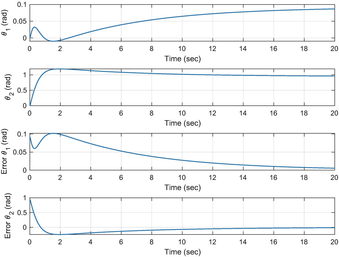
SCARA robot angles showing the transient response.
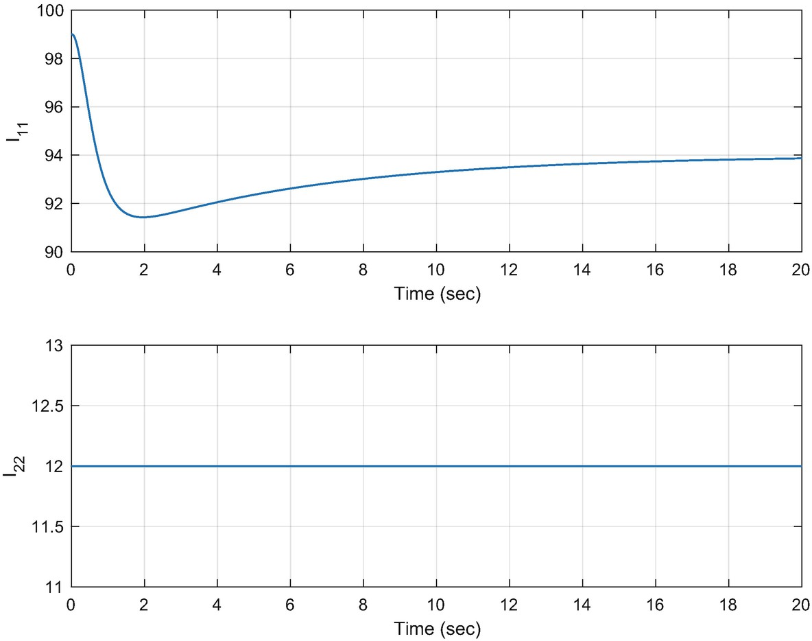
SCARA robot inertia as the arm moves.
After the simulation is done, the script runs an animation of the arm motion. Both 2D plots and the 3D animation are needed to debug the controller and for production runs.
The same script could be extended to show a sequence of commands to the arm.
8.6 Summary
This chapter has demonstrated how to write the dynamics and implement a simple control law for a two-link manipulator, the SCARA robot. We have implemented coupled nonlinear equations in the right-hand side with the simple controller developed in the previous chapter. The format of the simulation is very similar to the double integrator. There are more sophisticated ways of performing this control that would take into account the coupling between the links, which can be added to this framework. We have not implemented any constraints on the motion or the control torque.
Chapter Code Listing
File | Description |
DrawSCARA | Draw a SCARA robot arm |
RHSSCARA | Right-hand side of the SCARA robot arm equations |
SCARADataStructure | Initialize the data structure for all SCARA functions |
SCARAIK | Generate SCARA states for the desired end effector position and angle |
SCARARobotSim | SCARA robot demo |