© Michael Paluszek and Stephanie Thomas 2020
M. Paluszek, S. ThomasMATLAB Recipeshttps://doi.org/10.1007/978-1-4842-6124-8_11

11. Chemical Processes

Michael Paluszek1   and Stephanie Thomas2
(1)
Princeton, NJ, USA
(2)
Princeton Junction, NJ, USA
 

In chemical engineering, the production of chemicals needs to be modeled and the production process controlled. Our example will be a simple process in which the pH of a mixed solution needs to be controlled. This problem is interesting because the process is highly nonlinear and the sensor model does not have an explicit solution for the pH output. Modeling the sensor will require the use of the numerical solver fzero.

The specific chemical process we will study consists of an acid (HNO3) stream, a buffer (NaHCO3) stream, and a base (NaOH) stream that are mixed in a stirred tank.1 This is based on a bench-scale experiment developed at the University of California, Santa Barbara (UCSB), to study chemical process control.2 Figure 11.1 shows a diagram of the system, with three incoming streams q1, q2, and q3, and a valve to the output stream q4, where we will measure the pH. The goal will be to achieve a neutral pH.
../images/335353_2_En_11_Chapter/335353_2_En_11_Fig1_HTML.jpg
Figure 11.1

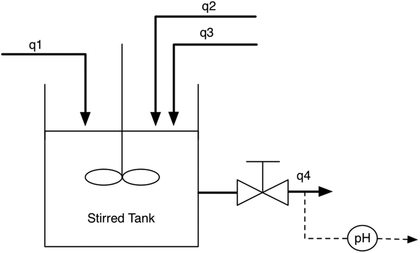
Chemical mixing problem.

11.1 Modeling the Chemical Mixing Process

Problem

We want to model the chemical process consisting of an acid stream, a buffer stream, and a base stream that are mixed in a stirred tank.

Solution

We model the chemical equilibria by adding two reaction invariants for each inlet stream and write the dynamical equations using the invariants. These are coded in a right-hand-side function that also defines the model data structure.

How It Works

Reaction invariants are quantities whose values do not change during a reaction. Each is a combination of chemicals that do not vary. Our inputs are nitric acid (HNO3), sodium bicarbonate or baking soda (NaHCO3), and sodium hydroxide or lye (NaOH). There is a pair of invariants for each input stream i. The two reaction invariants W a and W b are

$$displaystyle egin{aligned} egin{array}{rcl} W_{ai} & =&displaystyle [mathrm{H^+}]_i - [mathrm{OH^-}]_i - [mathrm{HCO_3^-}]_i - 2[mathrm{CO^=_3}]_i end{array} end{aligned} $$
(11.1)

$$displaystyle egin{aligned} egin{array}{rcl} W_{bi} & =&displaystyle [mathrm{H_2CO_3}]_i + [mathrm{HCO_3^-}]_i + [mathrm{CO^=_3}]_i end{array} end{aligned} $$
(11.2)
i = 1 is for the acid stream, i = 2 for the buffer stream, i = 3 for the base stream, and i = 4 is for the mixed effluent. These combinations of chemicals do not change. The amounts of the combinations may change. The dynamical equations for the effluent invariants are derived via mass balances to be

$$displaystyle egin{aligned} egin{array}{rcl} dot{W}_{a4} & =&displaystyle frac{1}{Ah}(W_{a1} - W_{a4})q_1 +frac{1}{Ah}(W_{a2} - W_{a4})q_2+frac{1}{Ah}(W_{a3} - W_{a4})q_3 end{array} end{aligned} $$
(11.3)

$$displaystyle egin{aligned} egin{array}{rcl} dot{W}_{b4} & =&displaystyle frac{1}{Ah}(W_{b1} - W_{b4})q_1 +frac{1}{Ah}(W_{b2} - W_{b4})q_2+frac{1}{Ah}(W_{b3} - W_{b4})q_3 end{array} end{aligned} $$
(11.4)
where q i is the volumetric flow rates for the i th stream, A is the cross-sectional area of the mixing tank, and h is the liquid level. The volumetric flow rates are inputs. The liquid level is governed by a differential equation:

$$displaystyle egin{aligned} dot{h} = frac{1}{A}left[q_1 + q_2 + q_3-C_v(h+z)^n
ight] end{aligned} $$
(11.5)
where C v is the valve coefficient, n is the valve exponent, and z is the vertical distance between the bottom of the mixing tank and the outlet of the effluent stream. We can measure h. Normally, we need to estimate the reaction invariants, but for this problem, we will assume they are measured. These equations are all first order and are therefore the state equations for the system. The flow rates are all multiplied by the states, meaning that their influence on the derivatives is a product of the states and the streams. The differential equations for the effluent invariants are singular when h = 0. This is because if the tank is empty, the flows have to be zero.

The resulting right-hand-side function, RHSpH, is shown in the following. This follows the format needed by our RungeKutta integrator (see Recipe 6.2), that is, RHS(t,x,d), with a tilde replacing the first input, as the dynamics are independent of time. Note the data structure which is defined and returned if there are no inputs. This model has quite a few parameters which are documented in the header.

RHSpH.m

../images/335353_2_En_11_Chapter/335353_2_En_11_Figa_HTML.gif

../images/335353_2_En_11_Chapter/335353_2_En_11_Figb_HTML.gif

The default values in the data structure are drawn from the data in the reference, with the exception of C v; this was neglected by the reference so we calculated a value for an equilibrium tank level.

../images/335353_2_En_11_Chapter/335353_2_En_11_Figc_HTML.gif

In this chapter, we are interested in control about an equilibrium point. We could rewrite the equations as linear equations in which each state and input is replaced with, for example

$$displaystyle egin{aligned} egin{array}{rcl} q_3 & =&displaystyle q_{30} + delta q_3 end{array} end{aligned} $$
(11.6)

$$displaystyle egin{aligned} egin{array}{rcl} h & =&displaystyle h_0 + delta h end{array} end{aligned} $$
(11.7)
where δq 3 is small. We could then formally derive the linear control system. We will leave that for the interested reader and just go ahead and implement a linear control system.

11.2 Sensing the pH of the Chemical Process

Problem

The pH sensor is modeled by a nonlinear equation that cannot be solved explicitly for pH.

Solution

Use the MATLAB fzero function to solve for pH.

How It Works

The equation for pH is1

$$displaystyle egin{aligned} 0 = W_{a4} + 10^{left(mathrm{pH}-14
ight)} -10^{-mathrm{pH}}+ W_{b4}frac{1 + 2	imes 10^{left(mathrm{pH}-pK_2
ight)} }{1 + 10^{left(pK_1 -mathrm{pH}
ight)}+ 10^{left(mathrm{pH}-pK_2
ight)}} end{aligned} $$
(11.8)
Recall that W a4 and W b4 are the reaction invariants for the mixed effluent as defined in Recipe 11.1. pK 1 and pK 2 are the base-10 logarithms of the H2CO3 and 
$$mathrm {HCO_3^-}$$
disassociation constants.

$$displaystyle egin{aligned}pK_{a} = -log_{10}K_{a}end{aligned}$$

The function that generates the measurement is PHSensor. Its inputs are two of the states of the system, W A4 and W B4, and the dissociation constants.

PHSensor.m

../images/335353_2_En_11_Chapter/335353_2_En_11_Figd_HTML.gif

The body of PHSensor calls fzero to compute the pH. This requires an objective function that will be searched for a zero near the input point. We use a neutral pH of 7.0 as the initial condition for the optimization. We could have warm started the function by using the last value that was computed. This is a good approach if the inputs don’t change quickly. The function is vectorized for multiple input states, computing a square matrix of pH with the combinations of W a4 and W b4.

../images/335353_2_En_11_Chapter/335353_2_En_11_Fige_HTML.gif

TIP

Use fzero to solve for the zero point for complex single equations. Use fminzero for sets of equations with multiple values to be found that minimized the function.

Notice that as per our usual pattern, we have defined a data structure d for passing data to the sensor model. Our two parameters are pK 1 and pK 2.

../images/335353_2_En_11_Chapter/335353_2_En_11_Figf_HTML.gif

Equation 11.8 is embodied in the subfunction Fun which is passed to fzero.

../images/335353_2_En_11_Chapter/335353_2_En_11_Figg_HTML.gif

We include a demo in the function as suggested in the best practices described in the style recipes. The demo specifies a range of values for the states – the invariants – based on the numbers in the reference.

../images/335353_2_En_11_Chapter/335353_2_En_11_Figh_HTML.gif

The results are plotted at the end of the main function using mesh. The mesh is the default plot.

../images/335353_2_En_11_Chapter/335353_2_En_11_Figi_HTML.gif

The plotting uses the mesh function. It is important to remember that the rows of p correspond to W a4 and the columns to W b4. Columns are x and rows are y in the mesh plot. Figure 11.2 shows the mesh plot and also the alternative surf plot (with 'edgecolor' set to 'none'). Note the two MATLAB commands:
../images/335353_2_En_11_Chapter/335353_2_En_11_Fig2_HTML.jpg
Figure 11.2

surf and mesh plots of the pH sensor output.

../images/335353_2_En_11_Chapter/335353_2_En_11_Figj_HTML.gif

Always use the on to be certain that the commands are executed rather than toggled. Otherwise, you can get unexpected results if you have just run another script or function with those commands.

Notice that the relationship between the pH and the reaction invariants is highly nonlinear. We would ideally like a relationship

$$displaystyle egin{aligned} pH = cleft[ egin{array}{l} W_{a4}\ W_{b4} end{array} 
ight]end{aligned} $$
(11.9)
where c is a 2-by-2 matrix with constant coefficients. This might be true in the flat regions but is not true in the “waterfall” region.

When using this function in a simulation, we need it to run as fast as possible, without any diagnostics installed for fzero. During debugging, however, you may need additional information. fzero can display information on each iteration by setting the Display option. For instance, with the 'iter' setting, it will print out information for each iteration. The updated fzero call is

../images/335353_2_En_11_Chapter/335353_2_En_11_Figk_HTML.gif

and the results for a single state are

../images/335353_2_En_11_Chapter/335353_2_En_11_Figl_HTML.gif

This was a very rapid solution as it is very near the starting point of 7.0. Note that fzero first found an interval containing a sign change, then searched for the zero. fzero can also output diagnostic information when complete instead of printing it during operation. For instance, if the call is

../images/335353_2_En_11_Chapter/335353_2_En_11_Figm_HTML.gif

then the output structure will be available, such as

../images/335353_2_En_11_Chapter/335353_2_En_11_Fign_HTML.gif

Note that the algorithm used, that is, bisection, is listed along with the total number of iterations and function evaluations. Consider a slight variation of the input state, lowering Wb4 to 4e −4 M. The number of iterations jumps significantly.

../images/335353_2_En_11_Chapter/335353_2_En_11_Figo_HTML.gif

Note in particular that viewing the diagnostic information for your problem can help confirm if your tolerances are suitable. Consider the final iterations of the previous case:

../images/335353_2_En_11_Chapter/335353_2_En_11_Figp_HTML.gif

The search pushed the function value all the way down to 5.4e-20, which may be more restrictive than needed. The default tolerances can be viewed by getting the default options structure using optimset.

../images/335353_2_En_11_Chapter/335353_2_En_11_Figq_HTML.gif

The default tolerance on the function value, TolX, is 2.2204e-16. Note that we passed in the name of the selected optimization routine, fzero, to optimset. The same can be done with fminbnd and fminsearch.

TIP

Use optimset with the name of the optimization function to get the default options structure.

Now consider that you want to evaluate how fzero is performing over a range of inputs. Assume that we create a separate function for Fun and make a script to record extra data from output during a run. Figure 11.3 shows a plot using pcolor of the resulting recorded function evaluations. We can see the rapid changes due to the nonlinearities of the model. The maximum number of function evaluations does not exceed 35.
../images/335353_2_En_11_Chapter/335353_2_En_11_Fig3_HTML.jpg
Figure 11.3

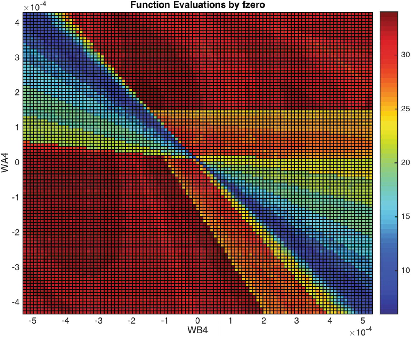
Function evaluations for the PHSensor algorithm.

The augmented code creating the plot is shown as follows:

SensorTest.m

../images/335353_2_En_11_Chapter/335353_2_En_11_Figr_HTML.gif

11.3 Controlling the Effluent pH

Problem

We want to control the pH level in the mixing tank when the flow of acid or base varies.

Solution

We will vary the base stream, i = 3, to maintain the pH. This means changing the value of q 3 using a proportional-integral controller. This will allow us to handle step disturbances.

How It Works

A proportional-integral controller is of the form

$$displaystyle egin{aligned} u = Kleft(1 + frac{1}{	au}int
ight)y end{aligned} $$
(11.10)
where u is the control, y is the measurement, τ is the integrator time constant, and K is the forward (proportional) gain. The control is u = q 3 and the measurement is y = pH. This makes this a single-input-single-output process. However, the connection between q 3 and pH involves three dynamical states h, W a4, and W b4, and the relationship between the states and pH is nonlinear. Another issue is that q 3 cannot be negative, that is, we cannot extract the base from the tank. This should not pose a problem if the equilibrium q 3 is high enough.

Despite these potential problems, this very simple controller will work for this problem for a fairly wide range of disturbances. The equilibrium value is input with a perturbation that has a proportional and integral term. The integral term uses a simpler Euler integration. The full script is described in the next recipe; here, we will call attention to the lines implementing the control.

The control variables are defined in the following. The pH set point is neutral, that is, a pH of 7. kF is the forward gain and tau is the time constant from Equation 11.10, set to 2 and 60 seconds, respectively. q3Set is the nominal set point for the base flow rate, taken from the reference.

PHProcessSim.m

../images/335353_2_En_11_Chapter/335353_2_En_11_Figs_HTML.gif

The following code snippet shows the implementation that takes place in a loop. The error is calculated as the difference between the modeled pH measurement and the pH set point. Note the Euler integration, where intErr is updated using simply the time step times the error. Note also that we have a flag, controlIsOn, which allows us to run the script in open loop, without the control being applied.

../images/335353_2_En_11_Chapter/335353_2_En_11_Figt_HTML.gif

To rigorously determine the forward gain and time constant for this problem, we would need to linearize the right-hand side for the simulation at the operating point and do a rigorous single-input-single-output control design that would involve Bode plots, root locus, and other techniques. This is beyond the scope of this book. For now, we simply select values which produce a reasonable response.

11.4 Simulating the Controlled pH Process

Problem

We want to simulate the stirred tank – mixing three streams: acid, buffer, and base – to demonstrate the control of the pH level. The base stream will be our control variable in response to perturbations in the buffer and acid streams.

Solution

We will write a script PHProcessSim with the controller starting at an equilibrium state. We will use the proportional-integral controller as derived in the previous recipe. We will structure the script to allow us to insert pulses in either or both the acid and buffer streams.

How It Works

Our disturbances d are deviations in q 1 and q 2:

$$displaystyle egin{aligned} d= left[ egin{array}{r} q_1\ q_2 end{array} 
ight] end{aligned} $$
(11.11)
which are the acid and buffer streams. The base stream is q 3 and the reaction invariants for the mixed effluent are W a4 and W b4. The system, as coded, is shown in Figure 11.4.
../images/335353_2_En_11_Chapter/335353_2_En_11_Fig4_HTML.jpg
Figure 11.4

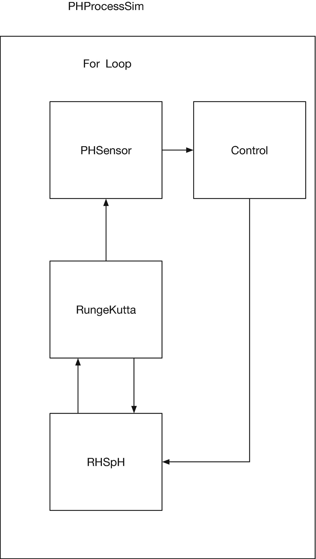
Block diagram of the mixing simulation representing the process in Figure 11.1.

We specify the user inputs to the script first. We are putting it into an equilibrium state and will investigate small disturbances from steady state. There is a flag, controlIsOn, for turning the control system on or off. The time step and duration are determined by iterating over a few values.

PHProcessSim.m

../images/335353_2_En_11_Chapter/335353_2_En_11_Figu_HTML.gif

The disturbances are generated as pulses to d.q1 and d.q2. The user parameters are the size and the start/stop times of the pulses. This setup will allow us to run cases similar to the reference.

../images/335353_2_En_11_Chapter/335353_2_En_11_Figv_HTML.gif

In the remainder of the script, we obtain the data structures defined in the previous recipes, specify the control parameters, and create the simulation loop. The measurements of the invariants are assumed to be exact; in practice, they need to be estimated. However, we should always test the controller under ideal conditions first, to understand its behavior without complications. The pH measurement is modeled using PHSensor from Recipe 11.2. The right-hand side for the process is defined in Recipe 11.1. Integration is performed using the RungeKutta defined in Chapter 7.

../images/335353_2_En_11_Chapter/335353_2_En_11_Figw_HTML.gif

../images/335353_2_En_11_Chapter/335353_2_En_11_Figx_HTML.gif

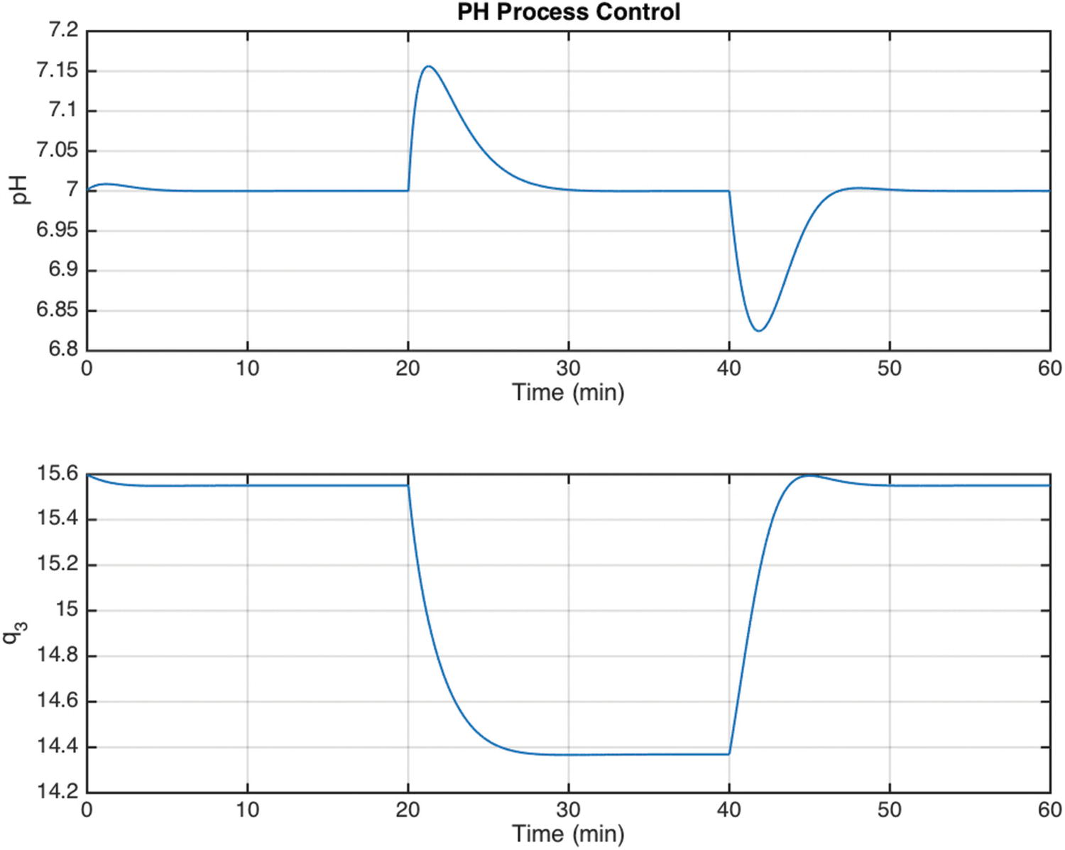
Now, we will give results for running this script with some different pulses. The nominal plot gives all three states, the measured pH, and the flow rates for the acid, base, and buffer streams. A more compact plot shows just the pH and the commanded value of q 3. We added a line in the plotting code to amend the plot title for an open loop response, so that if we run the script repeatedly, we can more easily identify the plots.

TIP

Use your control flags and string variables to customize the names of your plots.

Figure 11.5 shows the closed loop response with no disturbances at all, run for 30 simulated minutes. We can see that the values from the reference have not produced an exact equilibrium, but that the values achieved are quite close. The reaction invariant Wb4 changes by less than 0.005 × 10−4, the liquid level h by less than 0.1 cm, and the base flow rate q3 by about 0.05 ml/s. This is the equivalent to a very small step response. Note the settling time is about 5 minutes. These results give us confidence that we have coded the problem correctly. We will see this initial response in the following simulations, before the perturbations are applied.
../images/335353_2_En_11_Chapter/335353_2_En_11_Fig5_HTML.jpg
Figure 11.5

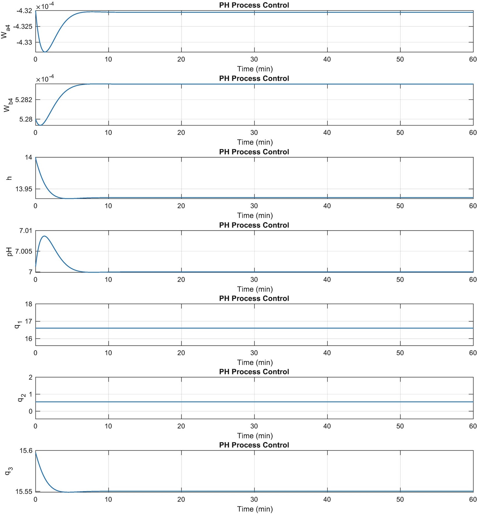
Closed loop response with no perturbations.

Next, Figure 11.6 shows the open loop response with a pulse of 0.65 ml/s in the buffer stream starting at 20 minutes and ending at 40 minutes. Note that the pH rises to nearly 7.4, and q 3 does in fact stay constant at our set point. Figure 11.7 shows the closed loop transients in the pH and base flow q 3. The pH rise is limited to less than 7.2, and the pH and base flow rate reach equilibrium within about 10 minutes of the start and end of the pulse. This compares favorably with the plots in the reference, which compare adaptive and nonadaptive nonlinear control schemes.
../images/335353_2_En_11_Chapter/335353_2_En_11_Fig6_HTML.jpg
Figure 11.6

Open loop response with a 0.65 ml/s pulse in q 2.

../images/335353_2_En_11_Chapter/335353_2_En_11_Fig7_HTML.jpg
Figure 11.7

Performance of the controller with a 0.65 ml/s pulse in q 2.

Figure 11.8 shows the transients with larger offset perturbations of 2 ml/s in both q 1 and q 2. The pulse in q 1 is applied from 5 to 15 minutes and the pulse in q 2 from 25 to 40 minutes. Figure 11.9 has plots of just the pH and control flow q 3.
../images/335353_2_En_11_Chapter/335353_2_En_11_Fig8_HTML.jpg
Figure 11.8

Performance of the controller with large perturbations of 2 ml/s in q 1 and q 2.

../images/335353_2_En_11_Chapter/335353_2_En_11_Fig9_HTML.jpg
Figure 11.9

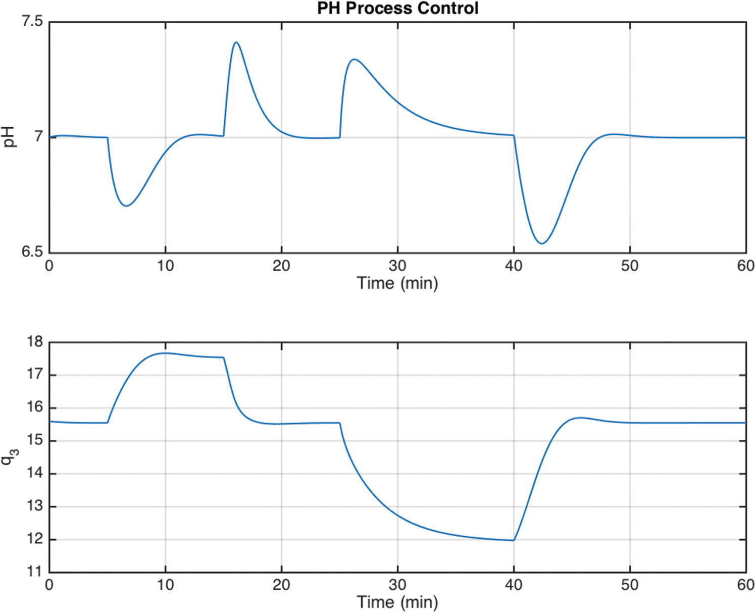
Larger plots of the q 1 /q 2 perturbation results.

Figure 11.10 shows the transients with a very large perturbation in q 2 of 8 ml/s from 5 to 35 minutes. The controller no longer works very well, with a much longer settling time than the previous examples and the base flow rate q 3 still dropping at the end of the pulse. A pulse value of 10 ml/s causes the simulation to “blow up” or produce imaginary values. It is always necessary to see the limits of the control performance in a nonlinear system.
../images/335353_2_En_11_Chapter/335353_2_En_11_Fig10_HTML.jpg
Figure 11.10

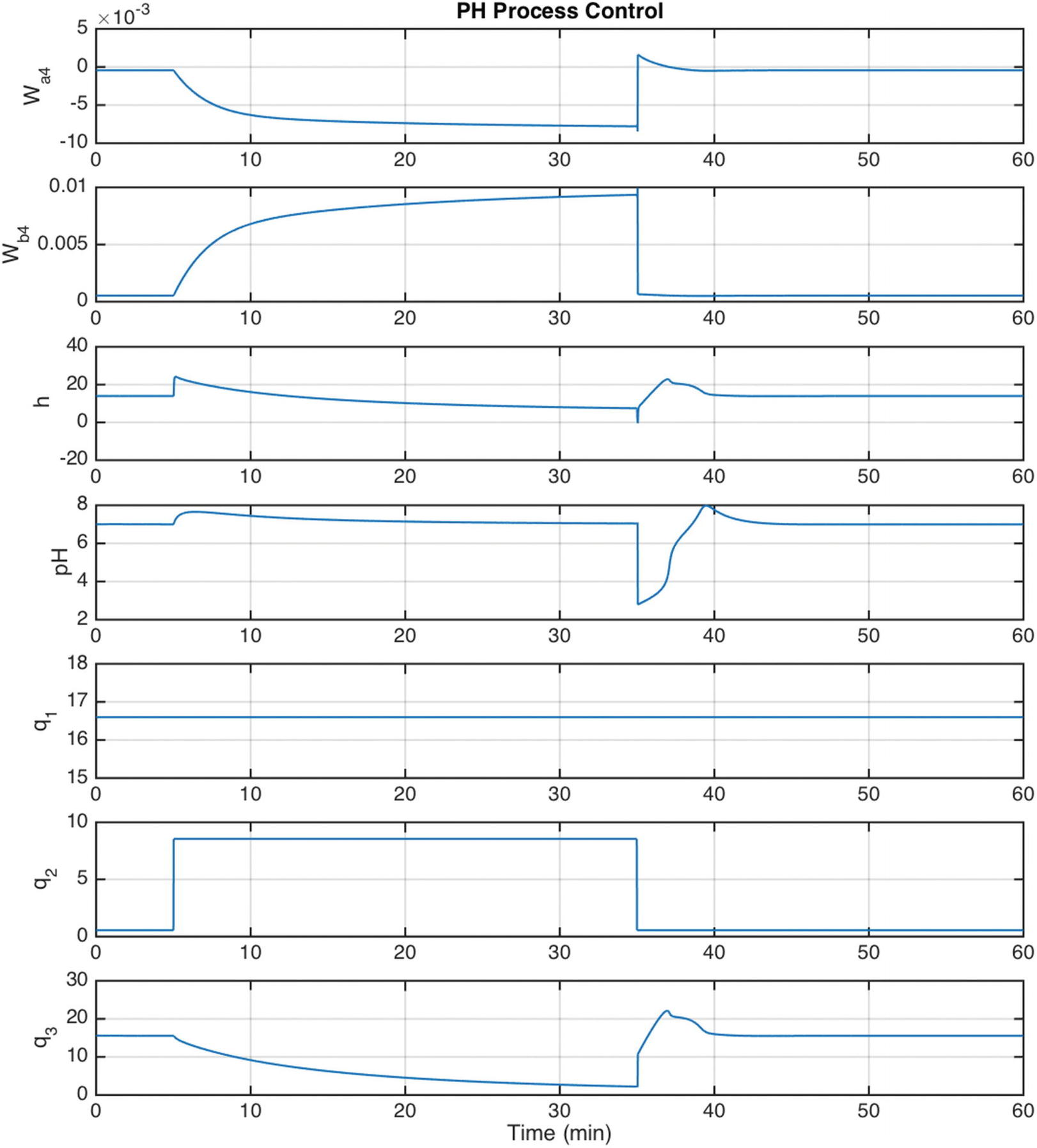
Performance of the controller with a very large perturbation (8 ml/s) in q 2.

Finally, since we are using a numerical optimization routine, it is instructive to profile the simulation to determine the proportion of the execution time spent on fzero. The Profiler can be accessed from the command window button called “Run and Time.” The summary from running our pH simulation is shown in Figure 11.11. Out of nearly 19 seconds spent in the simulation, fully 12.6 seconds are spent inside fzero itself. Only 4.4 seconds were spent integrating of which 3.4 seconds were spent in the right-hand side. The summary has hyperlinks to the individual functions, which are timed line by line. Figure 11.12 shows the time spent inside fzero, with percentages calculated in addition to absolute times. Our objective function, PHSensor>Fun, was called 56,131 times, taking only 1.27 seconds (10% of the execution time). Significant chunks of time were spent in sprintf and optimget.
../images/335353_2_En_11_Chapter/335353_2_En_11_Fig11_HTML.jpg
Figure 11.11

Profiler summary from the simulation.

../images/335353_2_En_11_Chapter/335353_2_En_11_Fig12_HTML.jpg
Figure 11.12

Profiler results for fzero.

TIP

Always do a run with the Profiler when you are implementing a numerical search or optimization routine. This gives you insight into the number of iterations used and any unsuspected bugs in your code.

In this case, there is not much optimization that can be done as most of the time is spent in fzero itself and not in our objective function, but we wouldn’t have known that without running the analysis. Whenever you are using numerical tools and have a script or function taking more than a second or two to run, analysis with Profiler is merited.

Summary
This chapter has demonstrated how to write the dynamics and implement a simple control law for a chemical process. The process is highly nonlinear, but we can control the process with a simple proportional-integral controller. The pH sensor does not have a closed form solution, and we use the MATLAB fzero function to find the pH from the invariants. We demonstrated the use of MATLAB plotting functions mesh and surf for showing three-dimensional data. We use our simulation script to evaluate the performance of the controller for a variety of conditions and run the script in the Profiler to analyze the time spent on the numerical routines. Table 11.1 lists the code developed in the chapter.
Table 11.1

Chapter Code Listing

File

Description

PHSensor

Model pH measurement of a mixing process

PHProcessSim

Simulation of a pH neutralization process

RHSpH

Dynamics of a chemical mixing process

SensorTest

Script to test the sensor algorithm

..................Content has been hidden....................

You can't read the all page of ebook, please click here login for view all page.
Reset
18.116.239.195