The purpose of this chapter is to provide an overview of MATLAB syntax and programming, highlighting features that may be underutilized by many users and noting important differences between MATLAB and other programming languages and IDEs. You should also become familiar with the very detailed documentation that is available from the MathWorks in the help browser. The Language Fundamentals section describes entering commands, operators, and data types.
MATLAB has matured a lot in the last two decades from its origins as a linear algebra package. Originally, all variables were double precision matrices. Today, MATLAB provides different variable types such as integers, data structures, object-oriented programming and classes, and integration with Java. The MATLAB application is a full IDE with an integrated editor, debugger, command history, and code analyzer and report capabilities. Engineers who have been working with MATLAB for many years may find that they are not taking advantage of the full range of capabilities now offered, and in this text we hope to highlight the more useful new features.
The first part of this chapter provides an overview of the most commonly used MATLAB types and constructs. We’ll then provide some recipes that make use of these constructs to show you some practical applications of modern MATLAB.
Brief Introduction to MATLAB
MATLAB is both an application and a programming language. It was developed primarily for numerical computing and is widely used in academia and industry. MATLAB was originally developed by a college professor in the 1970s to provide easy access to linear algebra libraries, and the MathWorks was founded in 1984 to continue the development of the product. The name is derived from MATrix LABoratory. Today, MATLAB uses the LAPACK libraries for the underlying matrix manipulations. Many toolboxes are available for different engineering disciplines; in this book, we will focus on features available only in the base MATLAB application.
The MATLAB application is a rich development environment for the MATLAB language. It provides an editor, command terminal, debugger, plotting capabilities, creation of graphical user interfaces, and more recently the ability to install third-party apps. MATLAB can interface with other languages including FORTRAN, C, C++, Java, and Python. A code analyzer and profiler are built-in. Extensive online communities provide forums for sharing code and asking questions.
- Command Window
– Terminal for entering commands and operating on variables in the base workspace. The MATLAB prompt is >>.
- Command History
– List of previously executed commands.
- Workspace display
– List of the variables and their values in the current workspace (application memory). Variables remain in the memory once created until you explicitly clear them or close MATLAB.
- Current Folder
– File browser displaying contents of the current folder and providing file system navigation. Recent versions of MATLAB can also display SVN status on configuration managed files.
- File details
– Panel displaying information on the file selected in the Current Folder panel.
- Editor
– Editor for m-files with syntax coloring and a built-in debugger. This can also display any type of text file and will recognize and appropriately color other languages including Java, C/C++, and XML/HTML.
- Variables editor
– Spreadsheet-like graphical editor for variables in the workspace.
- App Designer
– Application development window.
- Help browser
– Searchable help documentation on all MATLAB products and third-party products you have installed.
- Profiler
– Tool for timing code as it runs.
MATLAB desktop with the Command Window.
You can rearrange the components in the application window, moving, resizing, or hiding them, and save your own layouts. You can “undock” any component, moving it to its own window. You can also revert back to the default layout at any time or choose from several other available configurations. You can also hide the toolstrip to get more real estate for your windows. There are new capabilities to customize your interface with each version, so explore what’s new!
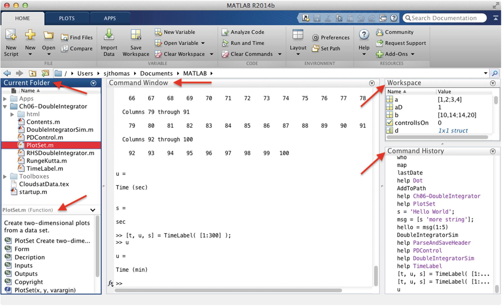
MATLAB file editor.
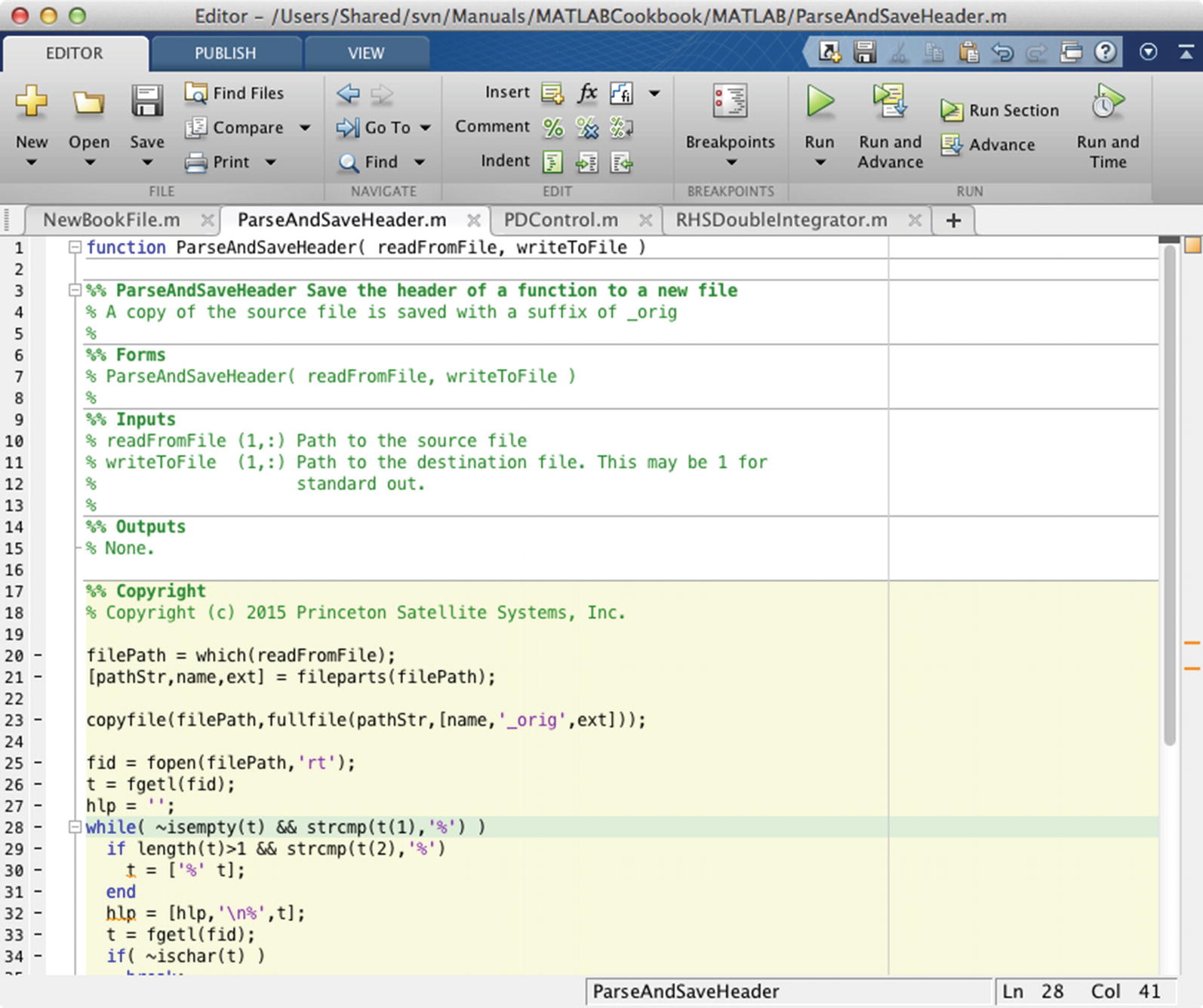
MATLAB help window.
By default, all variables in MATLAB are double precision matrices. You do not need to declare a type for these variables. Matrices can be multidimensional and are accessed using one-based indices via parentheses. You can address elements of a matrix using a single index, taken column-wise, or one index per dimension. Use square brackets to enclose the matrix data and semicolons to mark the end of rows. Use a final semicolon to end the line, or leave it off to print the result to the command line. To create a matrix variable, simply assign a value to it, like this 2x2 matrix a and 2x1 matrix b:
You can simply add, subtract, multiply, and divide matrices with no special syntax. The matrices must be the correct size for the linear algebra operation requested. A transpose is indicated using a single quote suffix, A’, and the matrix power uses the operator ̂.
Key Functions for Matrices
Function | Purpose |
|---|---|
zeros | Initialize a matrix to zeros |
ones | Initialize a matrix to ones |
eye | Initialize an identity matrix |
rand, randn, randi | Initialize a matrix of random numbers |
isnumeric | Identify a matrix or scalar numeric value |
isscalar | Identify a scalar value (a 1 x 1 matrix) |
size | Return the size of the matrix |
Character arrays are defined using single quotes. They can be concatenated using the same syntax as matrices, namely, square brackets. They are indexed the same way as matrices. Here is a short example of character array manipulation:
Use ischar to identify character variables. Also note that isempty returns TRUE for an empty array, that is, ''.
Since R2016b, MATLAB has also provided a string type defined using regular quotes. Some newer functions are designed to operate specifically on strings, but most work on both text types. If you concatenate strings using square brackets, they are maintained as separate elements in an array rather than combined as character arrays are. To append strings, use the “+” operator (see Recipe 1.5). isempty returns FALSE for an empty string, that is, ‘‘''; this creates a 1-by-1 string with no characters rather than an empty string.
Key Functions for Strings
Function | Purpose |
|---|---|
ischar | Identify a character array |
isstring | Identify a string |
char | Convert integer codes or cell array to character array |
sprintf | Write formatted data to a string |
strcmp, strncmp | Compare strings |
strfind | Find one string within another |
num2str, mat2str | Convert a number or matrix to a string |
lower | Convert a string to lowercase |
contains | Search for patterns in string arrays |
split | Split strings at whitespace |
Data structures in MATLAB are highly flexible, leaving it up to the user to enforce consistency in fields and types. You are not required to initialize a data structure before assigning fields to it, but it is a good idea to do so, especially in scripts, to avoid variable conflicts.
Replace

with
In fact, we have found it is generally a good idea to create a special function to initialize larger structures that are used throughout a set of functions. This is similar to creating a class definition. Generating your data structure from a function, instead of typing out the fields in a script, means you always start with the correct fields. Having an initialization function also allows you to specify the types of variables and provide sample or default data. Remember, since MATLAB does not require you to declare variable types, doing so yourself with default data makes your code that much clearer.
TIP
Create an initialization function for data structures.
You make a data structure into an array simply by assigning an additional copy. The fields must be in the same order, which is yet another reason to use a function to initialize your structure. You can nest data structures with no limit on depth.
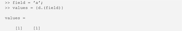
MATLAB now allows for dynamic field names using variables, that is, structName. (dynamicExpression). This provides improved performance over getfield, where the field name is passed as a string. This allows for all sorts of inventive structure programming. Take our data structure array in the previous code snippet, and let’s get the values of field a using a dynamic field name; the values are returned in a cell array.
Key Functions for Structs
Function | Purpose |
|---|---|
struct | Initialize a structure with or without fields |
isstruct | Identify a structure |
isfield | Determine if a field exists in a structure |
fieldnames | Get the fields of a structure in a cell array |
rmfield | Remove a field from a structure |
deal | Set fields in a structure to a value |
One variable type unique to MATLAB is the cell array. This is really a list container, and you can store variables of any type in elements of a cell array. Cell arrays can be multidimensional, just like matrices, and are useful in many contexts.
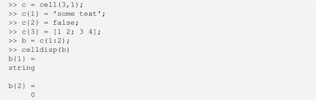
Cell arrays are indicated by curly braces, {}. They can be of any dimension and contain any data, including string, structures, and objects. You can initialize them using the cell function, recursively display the contents using celldisp, and access subsets using parentheses just like for a matrix. The following is a short example.
Using curly braces for access gives you the element data as the underlying type. When you access elements of a cell array using parentheses, the contents are returned as another cell array, rather than the cell contents. MATLAB help has a special section called Comma-Separated Lists which highlights the use of cell arrays as lists. The code analyzer will also suggest more efficient ways to use cell arrays, for instance:
Replace
a = {b{:} c};
with
a = [b {c}];
Cell arrays are especially useful for sets of strings, with many of MATLAB’s string search functions optimized for cell arrays, such as strcmp.
Key Functions for Cell Arrays
Function | Purpose |
|---|---|
cell | Initialize a cell array |
cellstr | Create cell array from a character array |
iscell | Identify a cell array |
iscellstr | Identify a cell array containing only strings |
celldisp | Recursively display the contents of a cell array |
A logical array is composed of only ones and zeros. You can initialize logical matrices using the true and false functions, and there is an islogical function to test if a matrix is logical. Logical arrays are outputs of numerous built-in functions, like isnan, and are often recommended by the code analyzer as a faster alternative to manipulating array indices. For example, you may need to set any negative values in your array to zero.
Replace
![]()
with
![]()
where x<0 produces a logical array with 1 where the values of x are negative and 0 elsewhere.
Key Functions for Logical Operations
Function | Purpose |
|---|---|
logical | Convert numeric values to logical |
islogical | Identify a logical array (composed of 1s and 0s) |
true | Return a true value (1) or array (M,N) |
false | Return a false value (0) or array (M,N) |
any | Return true if any value in the array is a nonzero number |
all | Return true if none of the values in the array is 0 |
and, or | Functional forms of element-wise operators & and | |
isnan, isinf, isfinite | Values testing functions returning logical arrays |
In general, variables defined in a function have a local scope and are only available within that function. Variables defined in a script are available in the workspace and, therefore, from the command line.
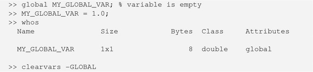
MATLAB has a global scope which is the same as any other language, applying to the base workspace and maintaining the variable’s value throughout the MATLAB session. Global variables are empty once declared, until initialized. The clear and clearvars functions each have flags for removing only the global variables. This is shown in the example below.
MATLAB has a unique scope that pertains to a single function, persistent. This is useful for initializing a function that requires a lot of data or computation and then saving that data for use in later calls. The variable can be reset using the clear command on the function, that is, clear functionName. This can also be a source of bugs so it is important to note the use of persistent variables in a function’s help comments, so you don’t get unexpected results when you switch models.
TIP
Use a persistent variable to store initialization data for subsequent function calls.
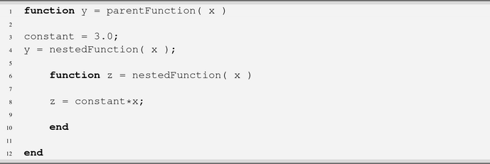
Variables can also be in scope for multiple functions defined in a single file, if the end keyword is used appropriately. In general, you can omit a final end for functions, but if you use it to wrap the inner functions, the functions become nested and can access variables defined in the parent function. This allows subroutines to share data without passing large numbers of arguments. The editor will highlight the variables that are so defined.
In the following example, the constant variable is available to the nested function inside the parent function.
Nested Function
Key Functions for Scope Operations
Function | Purpose |
|---|---|
persistent | Specify persistent scope for a variable in a function |
global | Specify global scope for a variable |
clear | Clear a function or variable |
who, whos | List variables in a workspace |
mlock, munlock | Lock (and unlock) a function or MEX-file which prevents it from being cleared |
Some common operators have special features in MATLAB, which we call attention to here.
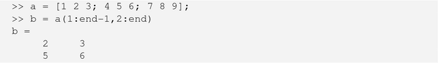
The colon operator for creating a list of indices in an array is unique to MATLAB. A single colon used by itself addresses all elements in that given dimension; a colon used between a pair of integers creates a list.
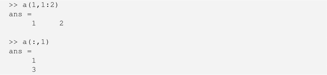
The colon operator applies to all variable types when accessing elements of an array: cell arrays, strings, data structure arrays.
The colon operator can also be used to create an array using an interval, as a shorthand to linspace. The interval and the endpoints can be doubles. Using it for matrix indices is really an edge case using a default interval of 1. For example, 0.1:0.2:0.5 produces 0.1 0.3 0.5.

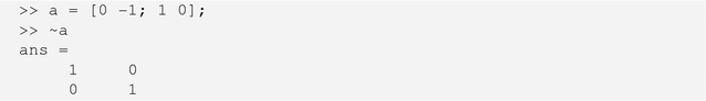
The tilde (∼) is the logical NOT operator in MATLAB. The output is a logical matrix of the same size as the input, with values of 1 if the input value is 0 and a value of 0 otherwise.
In newer versions, it also can be used to ignore an input or output to a function, and this is suggested often in the code analyzer as preferable to the use of a dummy variable.
![]()
By dot, we mean using a period with a standard arithmetic operator, like .* or .∖ or .̂. This is a special syntax in MATLAB used to apply an operator on an element per element basis over the matrices, instead of performing the linear algebra operation otherwise implied. This is also termed an array operation as opposed to a matrix operation. Since the matrix and array operations are the same for addition and subtraction, the dot is not required.
![]()
MATLAB is optimized for array operations. Using this syntax is a key way to reduce for loops in your MATLAB code and make it run faster. Consider the traditional alternative code:
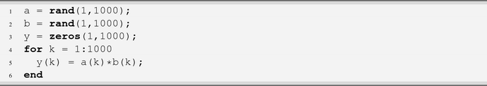
Even this simple example takes two to three times as long to run as the vectorized version shown above.
The end keyword serves multiple purposes in MATLAB. It is used to terminate for, while, switch, try, and if statements, rather than using braces as in other languages. It is also used to serve as the last index of a variable in a given dimension. Using end appropriately can make your code more robust to future changes in the size of your data.
Uniquely, MATLAB functions can have multiple outputs. They are specified in a comma-separated list just like the inputs. Additionally, you do not need to specify the data types of the inputs or outputs, and you can silently override the output types by assigning any data you want to the variables. Thus, a function can have an infinite number of syntaxes defined within a single file. Outputs must be assigned the names given in the signature; you cannot pass a variable to the return keyword.
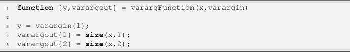
MATLAB provides helper functions for specifying a variable number of inputs or outputs, namely, varargin and varargout. These variables are cell arrays, and you access and assign elements using curly braces. Here is an example function definition:
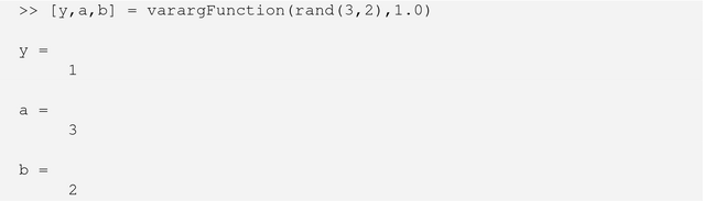
The following example demonstrates that the outputs were correctly assigned.
Using varargout and varargin
This allows you to accept unlimited arguments or parameter pairs in your function. It is up to you to create consistent forms for your function and document them clearly in the help comments.
You can also count the input and output arguments for a given call to your function using nargin and nargout and use this with logical statements or a switch statement to handle multiple cases.
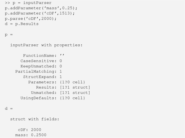
If you need very complex input handling, MATLAB now provides an inputParser class, which allows you to parse and validate an input scheme. You can define functions to validate the inputs, optional arguments, and predefine parameter pairs.
Function handles are pointers to functions. They are closely related to anonymous functions, which allow you to define a short function inline, and return the function handle. When you create a handle, you can change the input scheme and give values for certain inputs, that is, parameters. Using handles as inputs to integrators and similar routines is much faster than passing in a string variable of the function name.
In the following snippet, we create an anonymous function handle to myFunction with a different signature and a specific value for a. Note the use of the @, which designates a function handle. The handle can be evaluated with inputs just like a regular function.
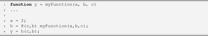
The handle h can be passed to a function such as an integrator that is expecting a signature with only two variables. You will also commonly use function handles to specify an events function for integrators or similar tools, as well as output functions that are called between major steps. Output functions can print information to the screen or a figure. See, for example, odeplot and odeprint.
In order to test if a variable is a function handle, you need to use the function handle class name with isa, that is:
![]()
Key Functions for Handles
Function | Purpose |
|---|---|
feval | Execute a function from a handle or string |
func2str | Construct a string from a function handle |
str2func | Construct a handle from a function name string |
isa | Test for a function handle |
While MATLAB defaults to doubles for any data entered at the command line or in a script, you can specify a variety of other numeric types, including single, uint8, uint16, uint32, uint64, logical (i.e., an array of booleans). The use of the integer types is especially relevant to using large data sets such as images. Use the minimum data type you need, especially when your data sets are large.
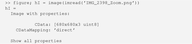
MATLAB supports a variety of formats including GIF, JPG, TIFF, PNG, HDF, FITS, and BMP. You can read in an image directly using imread, which can determine the type automatically from the extension, or fitsread. (FITS stands for Flexible Image Transport System, and the interface is provided by the CFITSIO library.) imread has special syntaxes for some image types, such as handling alpha channels for PNG, so you should review the options for your specific images. imformats manages the file format registry and allows you to specify handling of new user-defined types, if you can provide read and write functions.
You can display an image using either imshow, image, or imagesc, which scales the colormap for the range of data in the image.
For example, we use a set of images of cats in Chapter 7, Face Recognition. The following is the image information for a typical image:
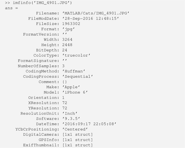
This is the metadata that tells the camera software, and image databases, where and how the image was generated. This is useful when learning from images as it allows you to correct for resolution (width and height) bit depth and other factors.
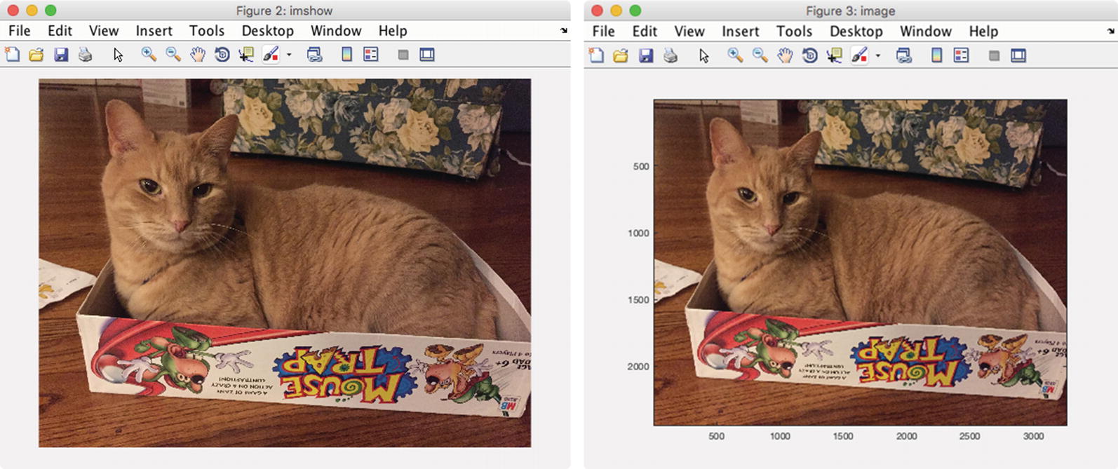
Image display options.
Key Functions for Images
Function | Purpose |
|---|---|
imread | Read an image in a variety of formats |
imfinfo | Gather information about an image file |
imformats | Determine if a field exists in a structure |
imwrite | Write data to an image file |
image | Display image from an array |
imagesc | Display image data scaled to the current colormap |
imshow | Display an image, optimizing figure, axes, and image object properties and taking an array or a filename as an input |
rgb2gray | Write data to an image file |
ind2rgb | Convert index data to RGB |
rgb2ind | Convert RGB data to indexed image data |
fitsread | Read a FITS file |
fitswrite | Write data to a FITS file |
fitsinfo | Information about a FITS file returned in a data structure |
fitsdisp | Display FITS file metadata for all HDUs in the file |
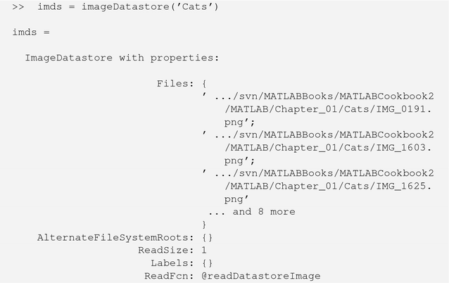
Datastores allow you to interact with files containing data that are too large to fit in memory. There are different types of datastores for tabular data, images, spreadsheets, databases, and custom files. Each datastore provides functions to extract smaller amounts of data that do fit in memory for analysis. For example, you can search a collection of images for those with the brightest pixels or maximum saturation values. We will use the directory of cat images included with the code as an example.
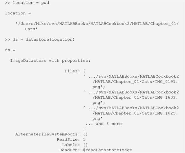
Once the datastore is created, you use the applicable class functions to interact with it. Datastores have standard container-style functions like read, partition, and reset. Each type of datastore has different properties. The DatabaseDatastore requires the Database Toolbox and allows you to use SQL queries.
Key Functions for Datastore
Function | Purpose |
|---|---|
datastore | Create a datastore |
read | Read a subset of data from the datastore |
readall | Read all of the data in the datastore |
hasdata | Check to see if there is more data in the datastore |
reset | Initialize a datastore with the contents of a folder |
partition | Excerpt a portion of the datastore |
numpartitions | Estimate a reasonable number of partitions |
ImageDatastore | Datastore of a list of image files |
TabularTextDatastore | A collection of one or more tabular text files |
SpreadsheetDatastore | Datastore of spreadsheets |
FileDatastore | Datastore for files with a custom format, for which you provide a reader function |
KeyValueDatastore | Datastore of key-value pairs |
DatabaseDatastore | Database connection, requires the Database Toolbox |
Tall arrays were introduced in R2016b. They are allowed to have more rows than will fit in memory. You can use them to work with datastores that might have millions of rows. Tall arrays can use almost any MATLAB type as a column variable, including numeric data, cell arrays, strings, datetimes, and categoricals. The MATLAB documentation provides a list of functions that support tall arrays. Results for operations on the array are only evaluated when they are explicitly requested using the gather function. The histogram function can be used with tall arrays and will execute immediately.
Tall Arrays
Analysis of Big Data with Tall Arrays
Functions That Support Tall Arrays
Index and View Tall Array Elements
Visualization of Tall Arrays
Extend Tall Arrays with Other Products
Tall Array Support, Usage Notes, and Limitations
Key Functions for Tall Arrays
Function | Purpose |
|---|---|
tall | Initialize a tall array |
gather | Execute the requested operations |
summary | Display summary information to the command line |
head | Access first rows of a tall array |
tail | Access last rows of a tall array |
istall | Check the type of the array to determine if it is tall |
write | Write the tall array to disk |
Key Functions for Sparse Matrices
Function | Purpose |
|---|---|
sparse | Create a sparse matrix from a full matrix or from a list of indices and values |
issparse | Determine if a matrix is sparse |
nnz | Number of nonzero elements in a sparse matrix |
spalloc | Allocate nonzero space for a sparse matrix |
spy | Visualize a sparsity pattern |
spfun | Selectively apply a function to the nonzero elements of a sparse matrix |
full | Convert a sparse matrix to full form |
Sparse matrices are a special category of matrix in which most of the elements are zero. They appear commonly in large optimization problems and are used by many such packages. The zeros are “squeezed” out, and MATLAB stores only the nonzero elements along with index data such that the full matrix can be recreated. Many regular MATLAB functions, such as chol or diag, preserve the sparseness of an input matrix.
Key Functions for Tables and Categoricals
Function | Purpose |
|---|---|
table | Create a table with data in the workspace |
readtable | Create a table from a file |
join | Merge tables by matching up variables |
innerjoin | Join tables A and B retaining only the rows that match |
outerjoin | Join tables including all rows |
stack | Stack data from multiple table variables into one variable |
unstack | Unstack data from a single variable into multiple variables |
summary | Calculate and display summary data for the table |
categorical | Arrays of discrete categorical data |
iscategorical | Create a categorical array |
categories | List of categories in the array |
iscategory | Test for a particular category |
addcats | Add categories to an array |
removecats | Remove categories from an array |
mergecats | Merge categories |
Categorical arrays allow for storage of discrete nonnumeric data, and they are often used within a table to define groups of rows. For example, time data may have the day of the week, or geographic data may be organized by state or county. They can be leveraged to rearrange data in a table using unstack. This is more efficient searching than elements of a cell array. See categorical and categories.
You can also combine multiple data sets into single tables using join, innerjoin, and outerjoin, which will be familiar to you if you have worked with databases.
You can access parts of a large MAT-file without loading the entire file into memory by using the matfile function. This creates an object that is connected to the requested MAT-file without loading it. Data is only loaded when you request a particular variable or part of a variable. You can also dynamically add new data to the MAT-file.
For example, we can load a MAT-file of neural net weights.
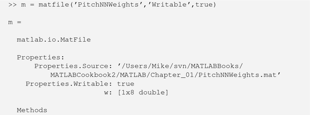
We can access a portion of the previously unloaded w variable or add a new variable name, all using this object m.
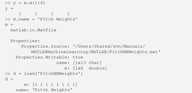
There are some limits to the indexing into unloaded data, such as struct arrays and sparse arrays. Also, matfile requires MAT-files using version 7.3, which is not the default for a generic save operation as of R2016b. You must either create the MAT-file using matfile to take advantage of these features or use the -v7.3’ flag when saving the file.
- Classes
– Classes, with properties and methods, can be defined using the classdef keyword in an m-file similar to writing a function. See also the properties, methods, and events keywords. See Chapter 6 for recipes using classes.
- Time series
– The timeseries object and the related tscollection object provide methods for associating data samples with timestamps. Plotting a timeseries object will use the stored time vector automatically.
- Map containers
– The map container allows you to store and look up data using a key which may be nonnumeric. This is an object instantiated via containers.Map.
The next part of this chapter provides recipes for some common tasks in modern MATLAB, like using different data types, adding help to your functions, loading binary data, writing to a text file, creating a MEX file, and parsing functions into “pcode.”
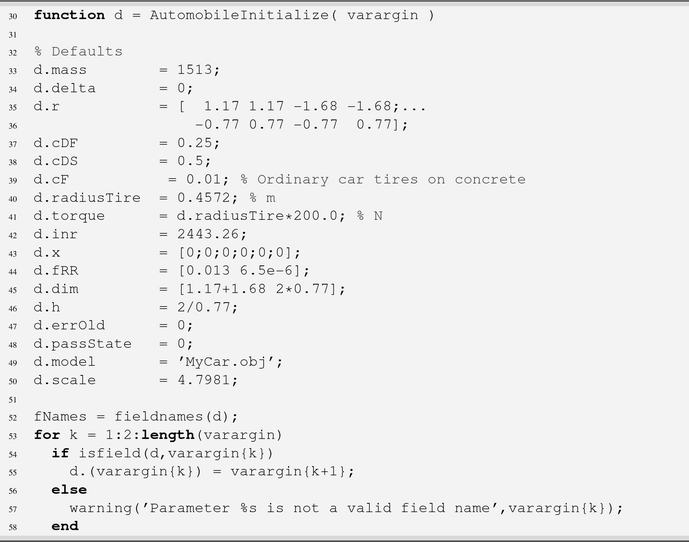
1.1 Initializing a Data Structure Using Parameters
It’s always a good idea to use a special function to define a data structure you are using as a type in your codebase, similar to writing a class but with less overhead. Users can then overload individual fields in their code, but there is an alternative way to set many fields at once: an initialization function which can handle a parameter pair input list. This allows you to do additional processing in your initialization function. Also, your parameter string names can be more descriptive than you would choose to make your field names.
Problem
We want to initialize a data structure so that the user clearly knows what they are entering.
Solution
The simplest way to implement the parameter pairs is using varargin and a switch statement. Alternatively, you could write an inputParser, which allows you to specify required and optional inputs as well as named parameters. In that case, you have to write separate or anonymous functions for validation that can be passed to the inputParser, rather than just write out the validation in your code.
How It Works
We will use the data structure developed for the automobile simulation as an example. The header lists the input parameters along with the input dimensions and units, if applicable.
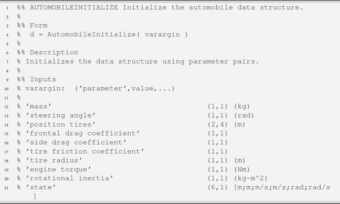
The function first creates the data structure using a set of defaults and then handles the parameter pairs entered by a user. After the parameters have been processed, two areas are calculated using the dimensions and the height.
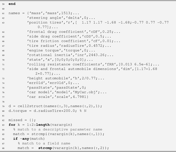

To perform the same tasks with inputParser, you add either an addRequired, addOptional, or addParameter call for every item in the switch statement. The named parameters require default values. You can optionally specify a validation function; in the following example, we use isNumeric to limit the values to numeric data.
In this case, the results of the parsed parameters are stored in a Results substructure.
1.2 Performing mapreduce on an Image Datastore
Problem
We discussed the datastore class in the introduction to the chapter. Now let’s use it to perform analysis on the full set of cat images using mapreduce, which is scalable to very large numbers of images. This involves two steps, first a map step that operates on the datastore and creates intermediate values and then a reduce step which operates on the intermediate values to produce a final output.
Solution
We create the datastore by passing in the path to the folder of cat images. We also need to create a map function and a reduce function, to pass into mapreduce. If you are using additional toolboxes like the Parallel Computing Toolbox, you would specify the reduce environment using mapreducer.
How It Works
First, create the datastore using the path to the images.
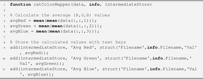
Second, we write the map function. This must generate and store a set of intermediate values that will be processed by the reduce function. Each intermediate value must be stored as a key in the intermediate key-value datastore using add. In this case, the map function will receive one image each time it is called. We call it catColorMapper, since it processed the red, green, and blue values for each image using a simple average.
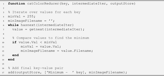
The reduce function will then receive the list of the image files from the datastore once for each key in the intermediate data. It receives an iterator to the intermediate datastore as well as an output datastore. Again, each output must be a key-value pair. The hasnext and getnext functions used are part of the mapreduce ValueIterator class. In this case, we find the minimum value for each key across the set of images.
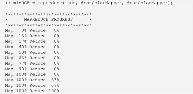
Finally, we call mapreduce using function handles to our two helper functions. Progress updates are printed to the command line, first for the mapping step and then for the reduce step (once the mapping progress reaches 100%).
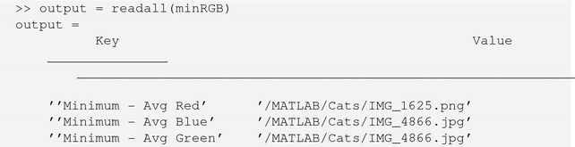
The results are stored in a MAT-file, for example, results_1_28-Sep-2016_16-28- 38_347. The store returned is a key-value store to this MAT-file, which in turn contains the store with the final key-value results.
You’ll notice that the image files are different file types. This is because they came from different sources. MATLAB can handle most image types quite well.
1.3 Creating a Table from a File
Often, with big data, we have complex data in many files. MATLAB provides functions to make it easier to handle massive sets of data. In this section, we will collect data from a set of weather files and perform a Fast Fourier Transform (FFT) on data from two years. First, we will write the FFT function.
Problem
We want to do Fast Fourier Transforms.
Solution
Write a function using fft and compute the energy from the FFT. The energy is just the real part of the product of the FFT output and its transpose.
How It Works
The following functions take in data y with a sample time tSamp and perform an FFT:
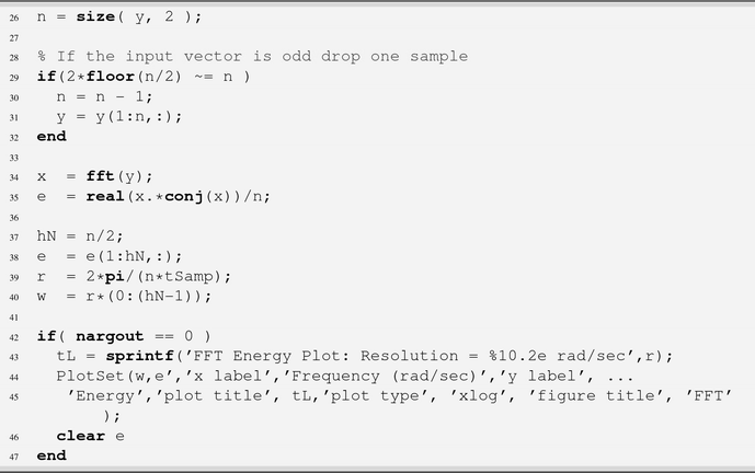
We get the energy using these two lines:
![]()
Taking the real part just accounts for numerical errors. The product of a number and its complex conjugate should be real.
The function computes the resolution. Notice it is a function of the sampling period and number of points.
![]()
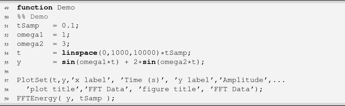
The built-in demo creates a series with a frequency at 1 rad/sec and a second at 2 rad/sec. The higher frequency one, with an amplitude of 2, has more energy as expected.
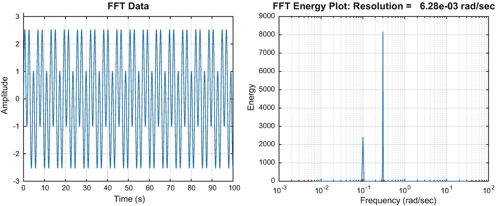
The input data for the FFT and the results.
1.4 Processing Table Data
Problem
We want to compare temperature frequencies in 1999 and 2015 using data from a table.
Solution
Use tabularTextDatastore to load the data and perform a Fast Fourier Transform on the data.
How It Works
First, let us look at what happens when we read in the data from the weather files.
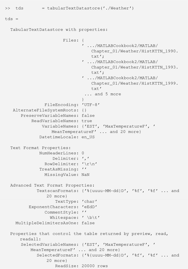
WeatherFFT selects the data to use. It finds all the data in the mess of data in the files. When running the script, you need to be in the same folder as WeatherFFT.
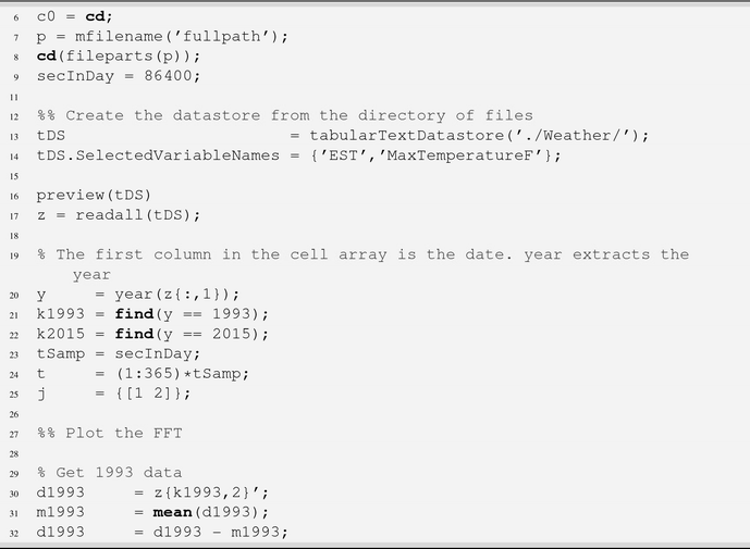
If the data does not exist, TabularTextDatastore puts NaN in the data points place. We happen to pick two years without any missing data. We use preview to see what we are getting.

1993 and 2015 data.
We get a little fancy with plotset. Our legend entries are computed to include the mean temperatures.

1.5 String Concatenation
In this next set of recipes, we will give examples of operations that work with strings but not with character arrays. Strings are a fairly new data type in MATLAB (since R2016b).
Problem
We want to concatenate two strings.
Solution
Create the two strings and use the “+” operator.
How It Works
You can use the + operator to concatenate strings. The result is the second string after the first.

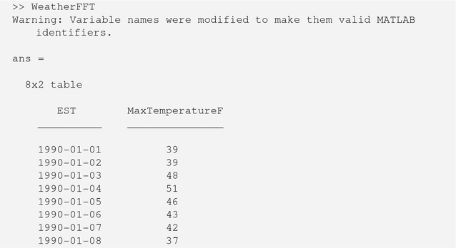
1.6 Arrays of Strings
Problem
We want any array of strings.
Solution
Create the two strings and put them in a matrix.
How It Works
We create the same two strings as shown earlier and use the matrix operator. If they were character arrays, we would need to pad the shorter with blanks to be the same size as the longer.
You could have used a cell array for this, but strings are more convenient.
1.7 Non-English Strings
Problem
We want to write a string in Japanese.
Solution
Copy the characters into a string array.
How It Works
Strings do not have to be in English. Copy any unicode characters into a MATLAB string.

The resulting string is
>> str
str =
1.8 Substrings
Problem
We want to get the portion of strings after a fixed prefix.
Solution
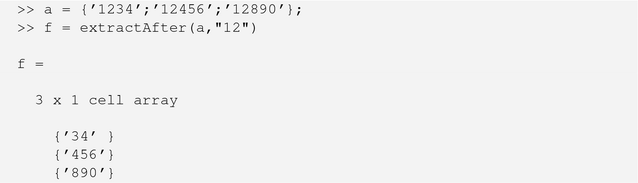
Create a string array and use extractAfter.
How It Works
Create a string array of strings to search and use extractAfter.

Most of the string functions work with char, but strings are a little cleaner. Here is the preceding example with cell arrays.
1.9 Using JSON-Formatted Strings
JSON (JavaScript Object Notation) is a lightweight data-interchange format used in JavaScript. MATLAB has functions for going to and from JSON. JSON covers all types of data. Encoding and decoding works with both cell arrays and data structures. This example code will get you started.

1.10 Creating Function Help
Problem
You need to document your functions so that others may use them, and you remember how they work in the future.
Solution
MATLAB provides a mechanism for providing command-line access to documentation about your function or script using the help command provided you put the documentation in the right place.
How It Works
The comments you provide at the top of your function file, called a header, become the function help. The help can be printed at the command line by typing help MyFunction. While we will cover the style and format of these comments in the next chapter, we draw your attention to the functionality here.
The help comments can go either above or below the declarative line of your function. If you include the words “see also” in your comments followed by the names of additional functions, MATLAB will helpfully supply links to those functions’ help. All comments are printed until the first blank line is reached.
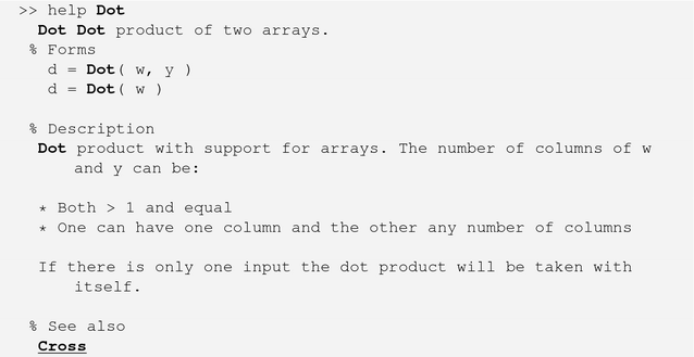
Consider the help for a function that calculates a dot product. The first line should be a single sentence description of the function, which is utilized by lookfor. If you insert your function name in all capital letters, MATLAB will automatically replace it with the true case version when printing the help. Your comments might look like this:

When printed to the command line, MATLAB will remove the percent signs and just display the text, like this:
You can link to additional help documentation attached to subfunctions in your file. (Subfunctions are visible to other functions in the same file, but not outside the file in which they are defined. However, you can output a handle to a subfunction.) This can be handy for providing more detailed examples or descriptions of algorithms. In order to do so, you have to embed an HTML link in your help comments, for example:
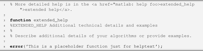
This typesets in the Command Window as
More detailed help is in the extended help.
MATLAB also provides the capability for you to create HTML help for your functions that will appear in the help browser. This requires the creation of XML files to provide the content hierarchy. See the MATLAB help topic Display Custom Documentation and the related recipe in the next chapter.
You can also run help reports to identify functions which are missing help or missing certain sections of help such as a copyright notice. To learn how to launch this report on your operating system, see the help topic Check Which Programs Have Help.
1.11 Locating Directories for Data Storage
Problem
A variety of demos and functions in your toolbox generate data files, and they end up all over your file system. You can’t use an absolute path on your computer because the code is shared among multiple engineers.
Solution
Use mfilename to save files in the same location as the generating file or to locate a dedicated data directory that is relative to your file location.
How It Works
It’s easy to sprinkle save commands throughout your scripts, or print figures to image files, and end up with files spread all over your file system. MATLAB provides a handy function, mfilename, which can provide the path to the folder of the executing m-file. You can use this to locate a data folder dedicated to either input files or output files for your routine. This uses the MATLAB functions fileparts and fullfile.
For example, to save an output MAT-file in the same location as your function or script:
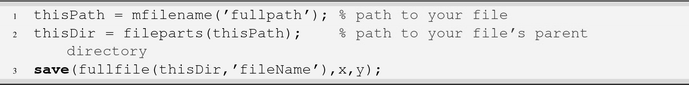
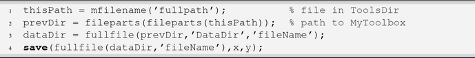
To save an output to a dedicated directory, you only need an additional call to fileparts. In this case, the directory is called DataDir. Say, for example, that your function is located in ToolsDir at the same level as DataDir in MyToolbox:
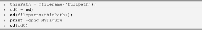
If you are printing images, you can either use the functional form of print as with save or change the path to the directory you want. You should save the current directory and return there when your script is complete.
Key Functions for Path Operations
Function | Purpose |
|---|---|
mfilename | Name and, optionally, full path to the current executing m-file |
fileparts | Divide a path into parts (directory, filename, extension) |
fullfile | Create a system-dependent filename from parts |
cd | The current directory |
path | The current MATLAB path |
1.12 Loading Binary Data from a File
Problem
You need to store data in a binary file, perhaps for input to another software program.
Solution
MATLAB provides low-level utilities for creating and writing to binary files including specifying the endianness.
How It Works
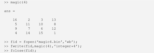
Reading and writing binary data do introduce some complexities beyond text files. Let’s start with MATLAB’s example of creating a binary file of a magic square. This demonstrates fopen, fwrite, and fread. The options for precision are specified in the help for fread. For example, a 32-bit integer can be specified with the MATLAB-style string 'int32' or the C-style string 'integer*4'.
Now, let’s try to read this data file back in. Since the data was stored as 32-bit integers, we have to specify this precision to get the data back.
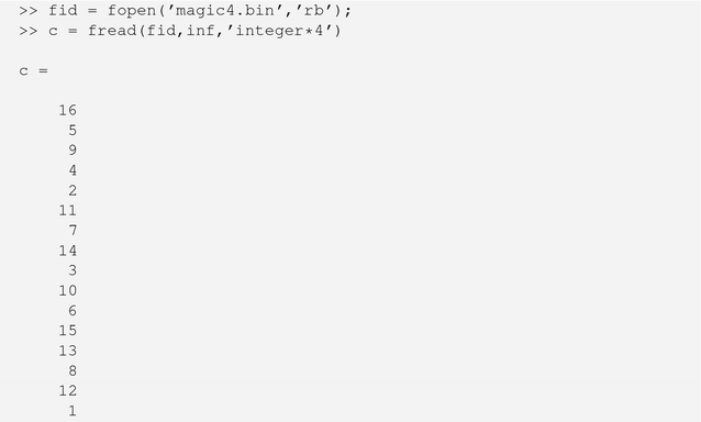
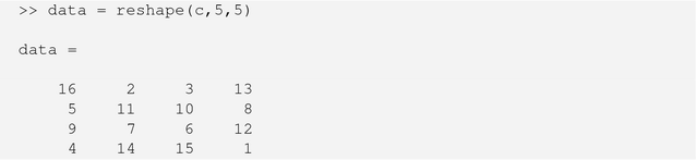
The shape of our matrix was not preserved, but we can see that the data was printed to the file in column-wise order. To fully recreate our data, we need to reshape the matrix.
If you need to specify the endianness of the data, you can do so in both fopen and fread. The local machine format is used by default, but you can specify the IEEE floating point with little endian byte ordering, the same with big ending ordering, and both with 64-bit long data type. This may be important if you are using binary data from an online source or using data on embedded processors.
For example, to write the same data in a big endian format, simply add the ’ieee-be’ parameter.

Key Functions for Binary Data
Function | Purpose |
|---|---|
fopen | Open a file in text or binary mode |
fwrite | Write to a file |
fread | Read the contents of a file |
fclose | Close the file |
1.13 Command-Line File Interaction
Problem
You have some unexpected behavior when you try to run a script MATLAB, and you suspect a function conflict among different toolboxes.
Solution
MATLAB provides functions for locating and managing files and paths from the command line.
How It Works
MATLAB has a file browser built-in to the Command Window, but it is still helpful to be familiar with the commands for locating and managing files from the command line. In particular, if you have a lot of toolboxes and files in your path, you may need to identify name conflicts.
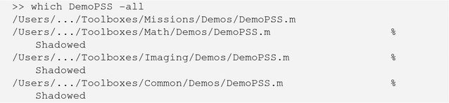
For example, if you get the wrong behavior or a strange error from a function and you recently changed your path, you may have a file shadowing it in your path. To check for duplicate copies of a function name, use which with the -all switch. Shadowed versions of the function will be marked. which can take a partial pathname.
To display the contents of a file at the command line, which is helpful if you need to see something in the file but don’t need to open the file for editing, use type, as in Unix.
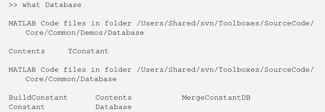
To list the contents of a directory, use what. A partial path can be used if there are multiple directories with the same name on your path. Specifying an output returns the results in a data structure array. MATLAB identifies which files are code, MAT-file, p-files, and so on. what is recursive and will return all directories with the given name anywhere in the path – useful if you use the same name of a directory for functions and demos, as follows:
Use exist to determine if a function or variable exists in the path or workspace. The code analyzer will prompt you to use the syntax with a second argument specifying the desired type, that is, ’var’, ’file’, ’dir’. The output is a numerical code indicating the type of the file or variable found.
Open a file in the editor from the command line using edit.
Load a MAT-file or ascii file using load. Give an output to store the data in a variable, or else it will be loaded directly into the workspace. For MAT-files, you can also specify particular variables to load.
![]()
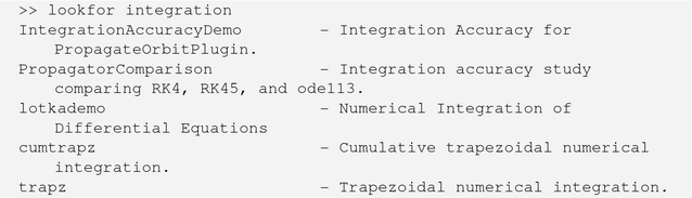
The final command-line function we will introduce is lookfor. This function searches through all help available on the MATLAB path for a keyword. The keyword must appear in the first line of the help, that is, the one-line help comment or “H1” line. The printed result looks like a Contents file and includes links to the help of the found functions. Here is an example for the keyword integration.
Key Functions for Command-Line Interaction
Function | Purpose |
|---|---|
which | Location of a function in the path |
what | List the MATLAB-specific files in the directory |
type | Display the contents of a file |
dbtype | Display the contents of a file with line numbers |
exist | Determine if a function or variable exists |
edit | Open a file in the editor |
load | Load a MAT-file into the workspace |
lookfor | Search help comments in the path for a keyword |
1.14 Using a MEX File to Link to an External Library
Problem
There is an external C++ library that you need to use for an application, and you would like to perform the analysis in MATLAB.
Solution
You can write and compile a special function in MATLAB using the C/C++ matrix API that will allow you to call the external library functions via a MATLAB function. This is called a MEX file.
How It Works
A MEX function is actually a shared library compiled from C/C++ or FORTRAN source code, and is callable from MATLAB. This can be used to link to external libraries such as GLPK, BLAS, and LAPACK. When writing a MEX function, you provide a gateway routine mexFunction in your code and use MATLAB’s C/C++ Matrix Library API. You must have a MATLAB-supported compiler installed on your machine.
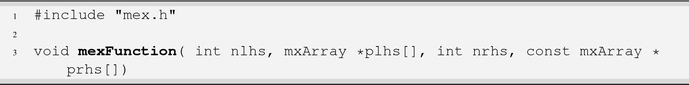
You can see that, as with regular MATLAB functions, you can provide multiple inputs and multiple outputs. mxArray is a C language type, actually the fundamental data type for all matrices in MATLAB, provided by the MATLAB API.
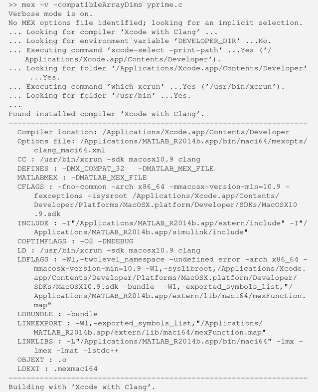
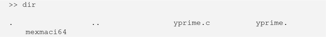
You use the mex function to compile your C, C++, or FORTRAN function into a binary. Passing the verbose flag, -v, provides verbose output familiar to C programmers. An extension such as “mexmaci64”, as determined on your system by mexext, is appended, and you can then call the function from MATLAB like any other m-file. For example, on Mac, MATLAB detects and uses Xcode automatically when compiling one of the built-in examples, yprime.c. This function “Solves simple 3 body orbit problem.” First, you need to copy the example into a local working directory.
![]()
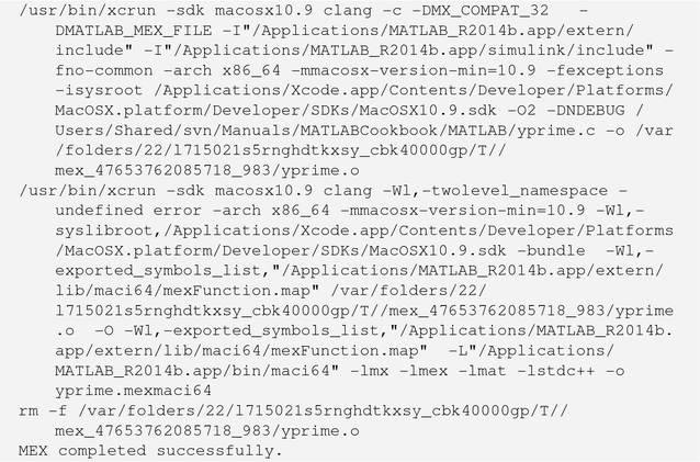
Some excerpts from the verbose compile are shown as follows:
Now, assuming you copied the source into an empty directory, if you now print the contents, you will see something like the following:
and you can run a test of the compiled library.

Writing MEX files is not for the faint of heart and requires substantial programming knowledge in the base language. In the preceding printout, you can see that the standard C++ library is included, but you need to provide links and include explicitly to other libraries you want to use. Note that your MEX-file will not have any function help, so it is a good idea to provide a companion m-file that supplies the help comments and calls your MEX function internally.
Provide a separate m-file with your MEX-file that contains help comments and, optionally, calls the MEX-file.
See the help articles including Components of MEX-File in MATLAB as well as the many included examples for help writing MEX-files. In the case of GLPK (GNU Linear Programming Kit), an excellent MEX file is available under the GNU public license. This was written by Nicolo Giorgetti and is maintained by Niels Klitgord. This is now available from SourceForge, http://glpkmex.sourceforge.net.
1.15 Protect Your IP with Parsed Files
Problem
You want to share files with customers or collaborators without compromising your intellectual property in the source code.
Solution
Create protected versions of your functions using MATLAB’s pcode function. Create a separate file with the help comments so users will have access to the documentation.
How It Works
The pcode function provides a capability to parse m-files into executable files with the content obscured. This can be used to distribute your software while protecting your intellectual property. A pcoded file on your path with a “p” extension, takes precedence over an m-file of the same name. Parsing an m-file is simple:
![]()
The only argument available is the -INPLACE flag to store the p-file in the same directory as the source m-file; otherwise, it will be saved to the current directory.
One difficulty you may encounter is that once you have parsed your functions and moved them into a new folder, you no longer have access to the function help you created. The command-line help is not implemented for pcoded files, and typing “help MyFunction” will no longer work. You have to create a separate .m file with the help comments as for MEX-files. We can write a function to extract the header from an m-file and save it. We will use fprintf for this, so it’s important that the header not contain any special characters like backslashes.

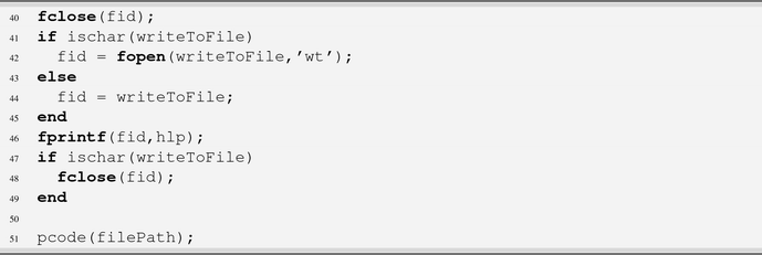
We save a copy of the m-file with a suffix _orig, to prevent unpleasant mistakes with deleted files. Note that we add a final comment at the end with the date the function was parsed.
1.16 Writing to a Text File
Problem
You need to write some information from MATLAB to a text file. One example is creating a template for new functions following a preferred format.
Solution
We will use fopen, fprintf, and fclose to open a new text file, print desired lines to it, and then close it. The input function is used to allow the user to enter a one-line summary of the function.
How It Works
MATLAB has a full set of functions for input and output, including writing to files. See help iofun for a detailed listing. You can write to text files, spreadsheets, binary files, XML, images, or zip files.
One useful example is creating a template for new functions for your company, following your preferred header format. This requires using fopen and fclose, and fprintf to print the lines to the file. The first input is the desired name of the new function. Note that fprintf will print to the command line if given a file ID of 1. We provide an option to do so with the second input, which is a boolean flag. We use the date function to get the current year for the copyright notice, which returns a string in the format ’dd-mmm-yyyy’; we use the string function strsplit to break the string into tokens. Using string indices would be an alternative. In addition, this demonstrates using input to prompt the user for a string, namely, a one-line description of the new function.
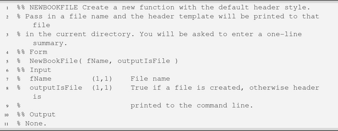
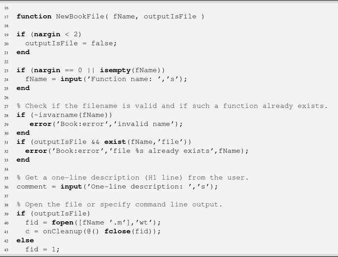
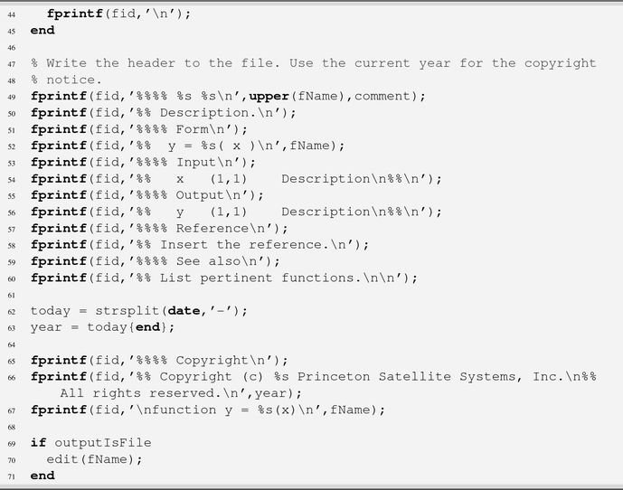
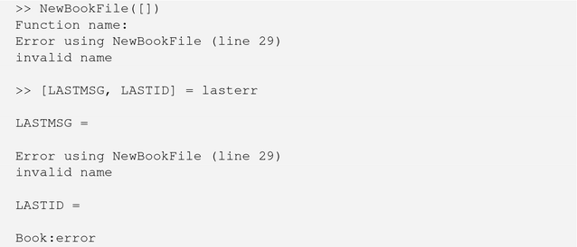
Note that this function checks for two errors, in the case of a bad function name and if a function with the same name already exists on the path. We use the two-input form of error where the first input is a message identifier. The message identifier is useful if an error is returned from a catch block. The message identifier can be verified using lasterr. For instance, if we fail to enter a valid function name when prompted, we can see the results of the first error.
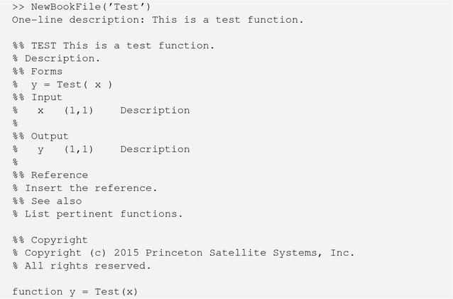
The function includes the ability to print the header to the Command Window, instead of creating a file, which is useful for testing – or if you went ahead and started with a blank file and need to add a header after the fact. This is accomplished by using 1 for the file identifier. Here is what the header will look like:
Key Functions for Interacting with Text Files
Function | Purpose |
|---|---|
fprintf | Print formatted text to a file |
strsplit | Split a string into tokens using a delimiter |
fgetl | Get one line of a file (until a newline character) |
input | Get string input from the user via the command line |
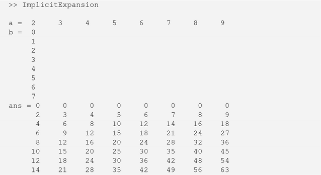
1.17 Using an Explicit Expansion
Problem
You need to use an explicit expansion.
Solution
Use the dot operator to produce an output with a higher dimension.
How It Works
Explicit expansion expands the dimensionality of the result automatically. In this case, we have an eight-element row and an eight-element column array. Prior to 2016b, these could not be multiplied. Now if you multiply them, it will automatically expand the dimensions of the results.
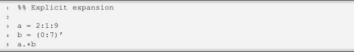
The results are shown in the following. The first element of b creates the first row of the output by multiplying every element of a. This is continued for the remaining elements of b.
1.18 Using a Script Subfunction
Problem
You need to write a script with a subfunction. This is useful when a script needs a function that is not of general utility. You can use this feature to avoid generating many separate function files that are only used in one place. We commonly use it for right-hand sides of simulation loops or for plotting methods needed to visualize data generated by the script.
Solution
We will add a subfunction to a script that provides the dynamics of a model.
How It Works
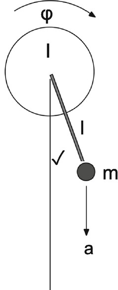
Simple slosh model.
The function Slosh.m provides a simple numerical model for fuel slosh on a spacecraft. The subfunction RHSSlosh starts with function and finishes with end. The script does not have an end before the function statement.
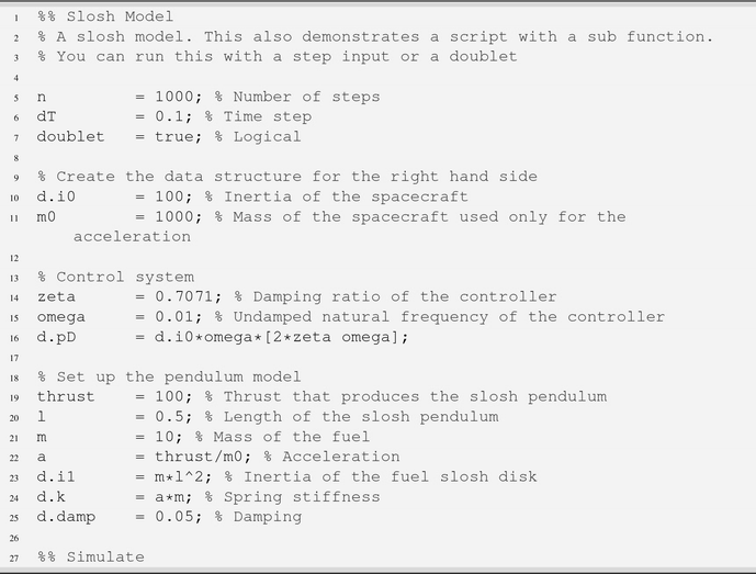
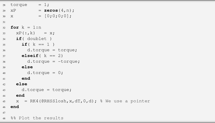
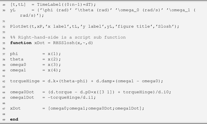
A few other things are worth noting. The subfunction RHSSlosh has an ∼, in the argument list because time is not used. We pass the names of the y-labels as a cell array using LaTeX symbols for the Greek letters. We set up the data structure, d, by just adding fields.
1.19 Using Memoize
Problem
You have a time-consuming process that you may have to do many times. However, the same inputs always result in the same outputs, so over many inputs, there is a duplication of computation.
Solution
We will use the memoize function. This is an optimization technique to speed up computation by storing the results of function calls in a cache, which can be accessed automatically when the same inputs are seen again. This is equivalent to storing a data table of outputs in a MAT-file, but faster.
How It Works
memoize stores the results in a buffer for later reuse. This is shown in the following script UseMemoize.m:

The results are

You can see that the second call is much faster, over 1000 times. This can be handier than storing the output. Note that a function to be memoized should not have any additional side effects, like affecting a global state, based on the inputs. Those side effects would not be repeated on additional calls to the function.
1.20 Using Java
Problem
We want to use MATLAB as a computational engine in Java.
Solution
We will use the MATLAB Engine.
How It Works
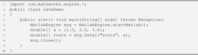
This will show how to use Java on Mac OS X. It will be similar on Linux and Windows. MATLAB provides a demo with a Java Swing GUI. First, get the demo function (or write your own Java).
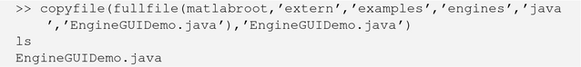
This is a fairly complex function. An example of using the engine in Java to compute roots is shown in the following. You define MATLABEngine.
You will need the MATLAB root to build your Java from Terminal.
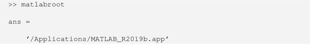
Open Terminal on Mac. cd (change directory) to the directory containing your Java. Compile using
![]()
Notice where we have the matlabroot. Run using

EngineGUIDemo.
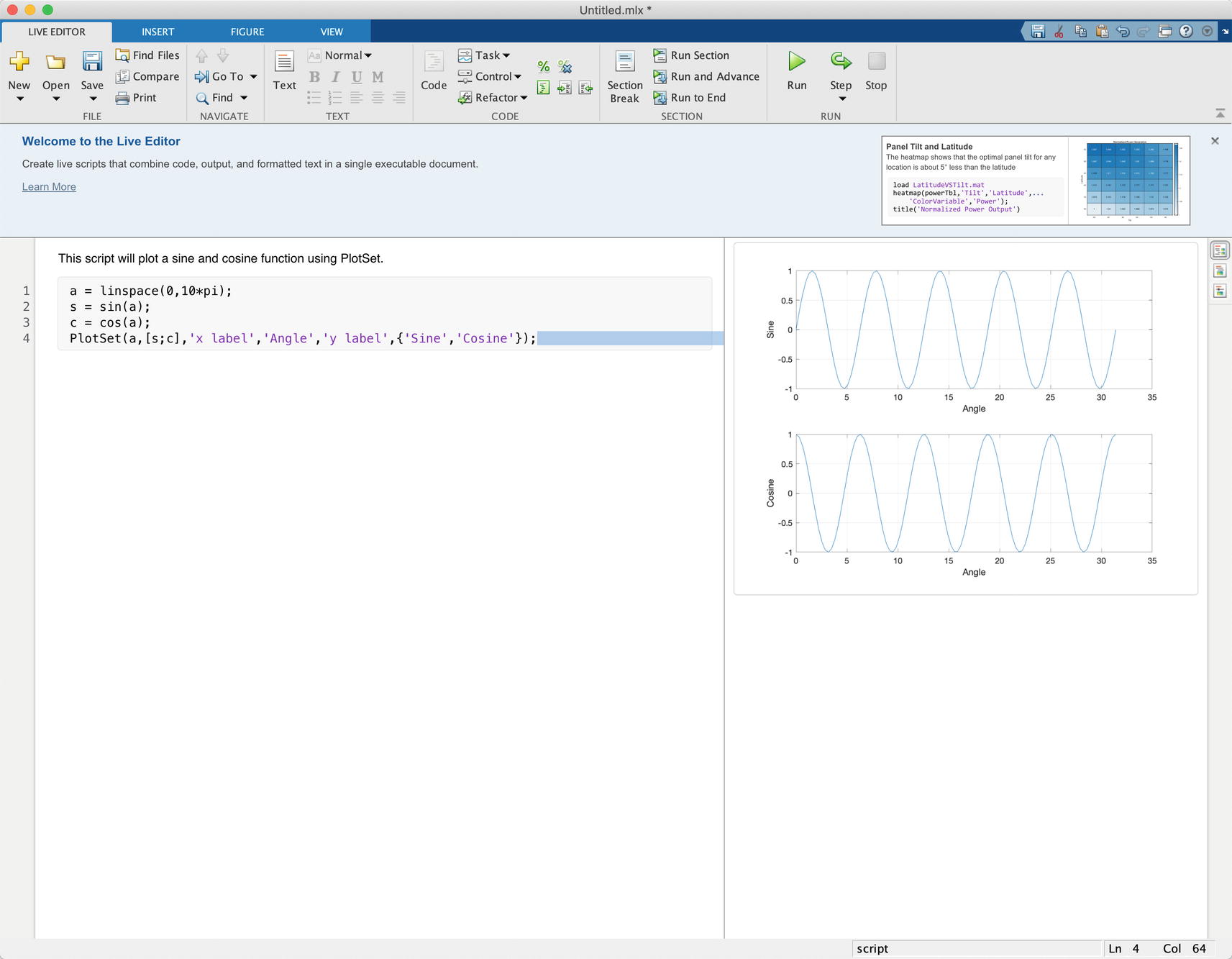
1.21 Creating Documents
Problem
We want to use MATLAB to create a document, combining text, code fragments, and plots. This can be a way to create a technical memo or document an analysis to be handed off to another engineer.
Solution
Use live scripts.
How It Works
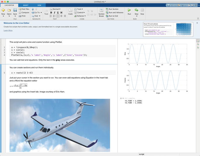
Live scripts allow you to create documents with active MATLAB code, text, equations, and images. Click New Live Script and you will see
Add text and code in the Live Editor tab.
To add equations and graphics, click the Insert tab. The equation editor is like the one in Microsoft Word.
Type
![]()
to open this document. If having trouble with running live scripts, you may need to disable any VPNs you have installed. Live scripts have many uses. For example, you can create interactive technical memos in which the reader can execute the MATLAB code needed to produce the results. This way, the reader can try different cases easily. You no longer need to list the MATLAB code used. Another use is interactive training.
1.22 MATLAB Online
Problem
We want to use MATLAB Online to work in MATLAB. This is using MATLAB through your web browser.
Solution
Set up MATLAB Online and a folder on your machine to access local folders.
How It Works
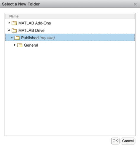
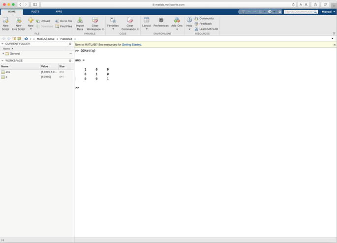
If you have a current MATLAB license, you can use MATLAB Online. On the MathWorks website, you can access MATLAB Online from the products page, under the Cloud Solutions category. The first step is to set up access to your local folder by downloading and executing MATLAB Drive Connector. Once that is done, drag the folders that you want to use into the MATLAB drive folder.
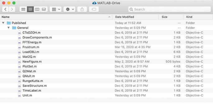
In this case, we dragged in the General folder from the code for this book. Go to the MATLAB Online web page and start the session.
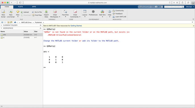
We already started the session. We created q and tried to run Q2Mat, which didn’t work.
You first need to click the folder with the down arrow in the toolbar to select the General folder.
This pop-up window will appear.
Fortunately, you don’t have to do this every time! Here is how it works when we return to the MATLAB Online.
This chapter reviewed the basic syntax for MATLAB programming. We highlighted differences between MATLAB and similar languages, like C and C++, in the language primer. Recipes give tips for efficient usage of key features, including writing to binary and text files. Tables at the end of each section highlight key functions you should have at your fingertips.
This chapter did not provide any information on using MATLAB’s computational tools, like integration and numerical search, as those will be left to subsequent chapters. Interacting with MATLAB graphics is also left to a later chapter.