© Michael Paluszek and Stephanie Thomas 2020
M. Paluszek, S. ThomasMATLAB Recipeshttps://doi.org/10.1007/978-1-4842-6124-8_9

9. Electric Motors

Michael Paluszek1   and Stephanie Thomas2
(1)
Princeton, NJ, USA
(2)
Princeton Junction, NJ, USA
 

We will model a three-phase permanent magnet motor driven by a direct current (DC) power source. This has three coils on the stator and permanent magnets on the rotor. This type of motor is driven by a DC power source with six semiconductor switches that are connected to the three coils, known as the A, B, and C coils. Two or more coils can be used to drive a brushless DC motor, but three coils are particularly easy to implement. This type of motor is used in many industrial applications today, including electric cars and robotics. It is sometimes called a brushless DC motor (BLDC) or a permanent magnet synchronous motor (PMSM).

Pulsewidth modulation is used for the switching because it is efficient; the switches are off when not needed. Coding the model for the motor and the pulsewidth modulation is relatively straightforward. In the simulation, we will demonstrate using two time steps, one for the simulation to handle the pulsewidths and one for the outer control loop. The simulation script will have multiple control flags to allow for debugging this complex system.

Figure 9.1 shows the big picture in this chapter. We will look at the motor model first (the AC motor block), then at the pulsewidth modulation (the SVPWM and three-phase inverter block). The controller is covered last. Each of these major functions is in a separated gray block.
../images/335353_2_En_9_Chapter/335353_2_En_9_Fig1_HTML.jpg
Figure 9.1

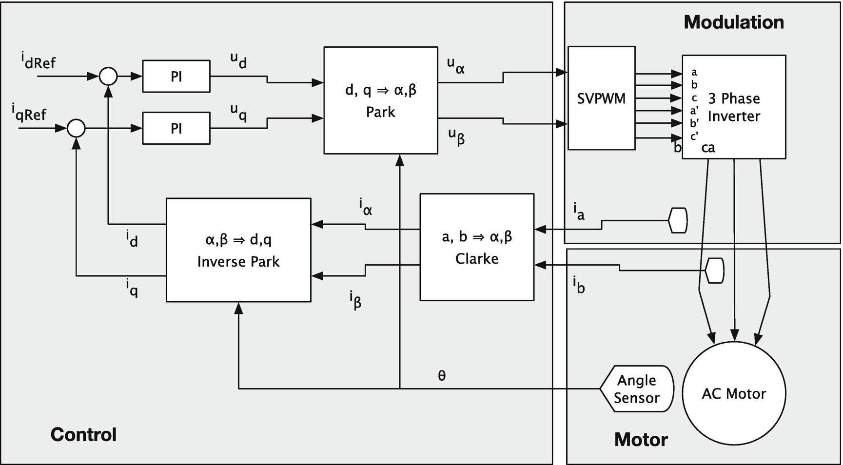
Motor controller. PI is the proportional-integral controller. PWM the is pulsewidth modulation. There are two current sensors measuring i a and i b and one angle sensor measuring θ.

9.1 Modeling a Three-Phase Brushless Permanent Magnet Motor

Problem

We want to model a three-phase permanent magnet synchronous motor in a form suitable for control system design. A conceptual drawing is shown in Figure 9.2. The motor has three stator windings and one permanent magnet on the rotor. The magnet has two poles or one pole pair. The coordinate axes are the a, b, and c on the stator, one axis at the center of each coil following the right-hand rule, and the (d,q) coordinates fixed to the magnet in the rotating frame. In motor applications, the axes represent currents or voltages, not positions like in mechanical engineering.
../images/335353_2_En_9_Chapter/335353_2_En_9_Fig2_HTML.jpg
Figure 9.2

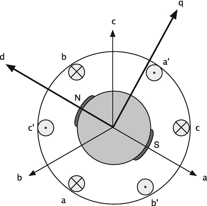
Motor diagram showing the three-phase coils a, b, and c on the stator and the two-pole magnet (N,S) on the rotor. The × means the current is going into the paper; the dot means it is coming out of the paper.

Solution

The solution is to model a motor with three stator coils and permanent magnets on the rotor. We have to model the coil currents and the physical state of the rotor.

How It Works

Permanent magnet synchronous motors use two or more windings in the stator and permanent magnets in the rotor. The rotor can have any even number of magnet poles. The phasing of the currents in the stator coils must be synchronized with the position of the rotor. Define the inductance matrix L, which gives the coupling between currents in different loops1:

$$displaystyle egin{aligned} L = frac{1}{d}left[ egin{array}{ccc} 2L_{ss} - L_m&L_m&L_m\ L_m&2L_{ss} - L_m&L_m\ L_m&L_m&2L_{ss} - L_m end{array} 
ight] end{aligned} $$
(9.1)
where

$$displaystyle egin{aligned} d = 2L^2_{ss} - L_{ss}L_m - L_m^2 end{aligned} $$
(9.2)
L m is the mutual inductance of the phase windings and L ss is the self-inductance. Self-inductance is the effect of a current in a loop on itself. Mutual inductance is the effect of the current in one loop on another loop. The three-phase current array, i, is

$$displaystyle egin{aligned} i = left[ egin{array}{l} i_{a}\ i_{b}\ i_{c} end{array} 
ight] end{aligned} $$
(9.3)
where i a is the phase A stator winding current, i b is the phase B current, and i c is the phase C current.
The phase voltage vector, u, is

$$displaystyle egin{aligned} u = left[ egin{array}{l} u_{a}\ u_{b}\ u_{c} end{array} 
ight] end{aligned} $$
(9.4)
where u a is the phase A stator winding voltage. The dynamical equations are a set of first-order differential equations and are

$$displaystyle egin{aligned} left[ egin{array}{l} dot{i}\ dot{omega}_{e}\ dot{	heta}_{e} end{array} 
ight] &= left[ egin{array}{rrr} -r_sL & 0 & 0\ 0 &-frac{b}{J}&0\ 0&1&0 end{array} 
ight] left[ egin{array}{l} i\ omega_{e}\ 	heta_{e} end{array} 
ight] + psi left[ egin{array}{l} -Lomega_{e}\ frac{p^2i^T}{4J}\ 0~0~0 end{array} 
ight] left[ egin{array}{l} cos	heta_{e}\ cos{}(	heta_{e} + frac{2pi}{3})\ cos{}(	heta_{e} - frac{2pi}{3}) end{array} 
ight] + left[ egin{array}{c} L\ 0~0~0\ 0~0~0 end{array} 
ight]u\ &quad + left[ egin{array}{l} 0\ frac{p}{2J}\ 0 end{array} 
ight]T_L end{aligned} $$
(9.5)
where ω is the rotor angular rate, θ is the rotor angle, p is the number of rotor poles, b is the viscous damping coefficient, r s is the stator resistance, ψ is the magnetic flux, T L is the load torque, and J is the rotor inertia. i and u are the phase winding 3-vectors shown earlier, and L is the 3-by-3 inductance matrix also shown earlier. Equation 9.5 is actually five equations in matrix form. The first three equations, for the current array i, are the electrical dynamics. The last two for ω e and θ e are the mechanical dynamics represented in electrical coordinates.
The driver circuitry is shown in Figure 9.3. It has six semiconductor switches. In this model, they are considered ideal, meaning they can switch instantaneously at any frequency we desire. In practice, switches will have a maximum switching speed and will have some transient response. Note that the motor is Y connected, meaning that the ends of the three-phase windings are tied together.
../images/335353_2_En_9_Chapter/335353_2_En_9_Fig3_HTML.jpg
Figure 9.3

Motor three-phase driver circuitry. The semiconductor switches shown in the diagram are IGBT (integrated gate bipolar transistors). The pulsewidth modulation block, SVPWM, is discussed in Recipe 9.3.

The right-hand-side code is shown in the following. The first output is the state derivative, as needed for integration. The second output is the electrical torque needed for the control. The first block of code defines the motor model data structure with the parameters needed by our dynamics equation. This structure can be retrieved by calling the function with no inputs. The remaining code implements Equation 9.5. Note the suffix M used for ω and θ, to reinforce that these are mechanical quantities; this distinguishes them from the electrical quantities which are related by p∕2, where p is the number of poles. The use of M and E subscripts is typical when writing software for motors.

The function returns a default data structure if no input arguments are passed to it. This is a convenient way for the designer of the code to give users a working starting point for the model. This way, the user only has to change parameters that are different from the default. It lets the user get up and running quickly.

The electrical torque is a second output argument. It is not used during numerical integration but is helpful when debugging the function. It is useful to output quantities that a user might want to plot too. MATLAB is helpful in allowing multiple outputs for a function.

RHSPMMachine.m

../images/335353_2_En_9_Chapter/335353_2_En_9_Figa_HTML.gif

../images/335353_2_En_9_Chapter/335353_2_En_9_Figb_HTML.gif

9.2 Controlling the Motor

Problem

We want to control the motor to produce a desired torque. Specifically, we need to compute the voltages to apply to the stator coils.

Solution

We will use field-oriented control with a proportional-integral controller to control the motor. Field-oriented control is a control method where the stator currents are transformed into two orthogonal components. One component defines the magnetic flux of the motor and the other defines the torque. The control voltages we calculate will be implemented using pulsewidth modulation of the semiconductor switches as developed in the previous recipe. Torque control is only one type of motor control. Speed control is often the goal. Robots often have position control as the goal. One could use torque control as an inner loop for either a speed controller or position controller.

How It Works

The motor controller is shown in Figure 9.1. This implements field-oriented control (FOC). FOC effectively turns the brushless three-phase motor into a commutated DC motor.

There are three electrical frames of reference in this problem. The first is the (a,b,c) frame which is the frame of the three-phase stator as in Figure 9.2. This is a time-varying frame. We next want to transform into a two-axis time-varying frame, the (α,β) frame, and then into a two-axis time-invariant frame, the (d, q) frame, which is also known as the direct-quadrature axes and is fixed to the permanent magnet. In our frames, each axis is a current. Since with a Y-connected motor the sum of the currents is zero:

$$displaystyle egin{aligned} 0 = i_a + i_b + i_c end{aligned} $$
(9.6)
we need only work with two currents, i a and i b.
The (d, q) to (α, β) transformation is known as the Forward Park transformation:

$$displaystyle egin{aligned} left[ egin{array}{r} u_alpha\ u_eta end{array} 
ight] = left[ egin{array}{rrr} cos	heta_e & -sin{	heta_e}\ sin	heta_e &cos	heta_e end{array} 
ight] left[ egin{array}{r} u_d\ u_q end{array} 
ight] end{aligned} $$
(9.7)
This transforms from the stationary d, q frame to the rotating (α, β) frame. θ e is in electrical axes and equals 
$$frac {1}{2}p,	heta _{M}$$
where p is the number of magnet poles. The Forward Clarke transformation for a Y-connected motor is

$$displaystyle egin{aligned} left[ egin{array}{r} u_alpha\ u_eta end{array} 
ight] = left[ egin{array}{rrr} 1 & 0\ frac{1}{sqrt{3}} &frac{2}{sqrt{3}} end{array} 
ight] left[ egin{array}{r} u_a\ u_b end{array} 
ight] end{aligned} $$
(9.8)

These two transformations are implemented in the functions ClarkeTransformation Matrix and ParkTransformationMatrix. They allow us to go from the time-varying (a,b,c) frame to the time-invariant, but rotating, (d,q) frame.

The equations for a general permanent magnet machine in the direct-quadrature frame are

$$displaystyle egin{aligned} egin{array}{rcl} u_q = r_s i_q + omega_e(L_d i_d + psi) +frac{dL_qi_q}{dt} end{array} end{aligned} $$
(9.9)

$$displaystyle egin{aligned} egin{array}{rcl} u_d = r_s i_d - omega_eL_q i_q +frac{d(L_di_d+ psi)}{dt} end{array} end{aligned} $$
(9.10)
where u are the voltages, i are the currents, r s is the stator resistance, L q and L d are the d and q phase inductances, ω e is the electrical angular rate, and ψ is the flux due to the permanent magnets. The electrical torque produced is

$$displaystyle egin{aligned} T_e = frac{3}{2}p((L_d i_d + psi) i_q - L_q i_q i_d) end{aligned} $$
(9.11)
where p is the number of pole pairs.
The torque equation is

$$displaystyle egin{aligned} T_e =T_L+ bomega_m + Jfrac{domega_m}{dt} end{aligned} $$
(9.12)
where b is the mechanical damping coefficient, T L is the external load torque, and J is the inertia, and the relationship between the mechanical and the electrical angular rate is

$$displaystyle egin{aligned} omega_e = pomega_m end{aligned} $$
(9.13)
The more pole pairs you have, the higher the electrical frequency. In a magnet surface mount machine with coils in slots, L d = L q ≡ L, and ψ and the inductances are not functions of time. The equations simplify to

$$displaystyle egin{aligned} egin{array}{rcl} u_q & =&displaystyle r_s i_q + omega_eL i_d + omega_epsi +Lfrac{di_q}{dt} end{array} end{aligned} $$
(9.14)

$$displaystyle egin{aligned} egin{array}{rcl} u_d & =&displaystyle r_s i_d - omega_eL i_q +Lfrac{di_d}{dt} end{array} end{aligned} $$
(9.15)
We control direct current i d to zero. If i d is zero, control is linear in i q. The torque is now

$$displaystyle egin{aligned} T_e = frac{3}{2}p psi i_q end{aligned} $$
(9.16)
Thus, the torque is a function of the quadrature current i q only. We can therefore control the electrical torque by controlling the quadrature current. The quadrature current is in turn controlled by the direct and quadrature phase voltages. The desired current 
$$i_q^{s}$$
can now be computed from the torque set point 
$$T_e^{s}$$
.

$$displaystyle egin{aligned} i_q^{s} = frac{2}{3} T_e^{s} / (p psi ) end{aligned} $$
(9.17)
We will use a proportional-integral controller to compute the (d,q) voltages. The proportional part of the control drives errors to zero. However, if there is a steady disturbance, there will be an offset. The integral part can drive an error due to such a steady disturbance to zero. Without the integral term, a steady disturbance will result in a steady error. A proportional-integral controller is of the form

$$displaystyle egin{aligned} u = Kleft(1 + frac{1}{	au}int
ight)y end{aligned} $$
(9.18)
where u is the control, y is the measurement, τ is the integrator time constant, and K is the forward (proportional) gain. Our control u will be the phase voltages, and our measurement y is the current error in the (d,q) frame.

$$displaystyle egin{aligned} u_{(d,q)} = -k_{F}left(i_{err} + frac{1}{	au}int i_{err} 
ight) end{aligned} $$
(9.19)
where

$$displaystyle egin{aligned} left[egin{array}{c}i_{d}\i_{q}end{array}
ight]_{err} = left[egin{array}{c}i_{d}\i_{q}end{array}
ight] - left[egin{array}{c}0\i_{q}^{s}end{array}
ight] end{aligned} $$
(9.20)

We now write a function, TorqueControl, that calculates the control voltages u (α,β) given the current state x. The state vector is the same as Recipe 9.1, that is, current i in the (a,b,c) frame plus the angle states θ and ω. We use the Park and Clarke transformations to compute the current in the (d,q) frame. We can then implement the proportional-integral controller with Euler integration. The function uses its data structure as memory – the updated structure d is passed back as an output. TorqueControl is shown as follows. This function will return a default data structure if no inputs are passed into the function.

TorqueControl.m

../images/335353_2_En_9_Chapter/335353_2_En_9_Figc_HTML.gif

../images/335353_2_En_9_Chapter/335353_2_En_9_Figd_HTML.gif

9.3 Pulsewidth Modulation of the Switches

Problem

In the previous recipe, we calculate the control voltages to apply to the stator. Now we want to take those control voltages as an input and drive the switches via pulsewidth modulation.

Solution

We will use the Space Vector Modulation to go from a rotating two-dimensional (α,β) frame to the rotating three-dimensional (a,b,c) stator frame, which is more computationally efficient than modulating in (a,b,c) directly.

How It Works

We will use Space Vector Modulation to drive the switches for pulsewidth modulation.2 This goes from (α,β) coordinates to switch states (a,b,c). Each node of each phase is either connected to ground or to +u. These values are shown in Figure 9.4. The six spokes in the diagram, as well as the origin, correspond to the eight discrete switch states.
../images/335353_2_En_9_Chapter/335353_2_En_9_Fig4_HTML.jpg
Figure 9.4

Space Vector Modulation in (α,β) coordinates. We determine which sector (in Roman numerals) we are in and then pick the appropriate vectors to apply so that they on average attain the desired voltage. The numbers in brackets are the normalized [α, β] voltages.

Table 9.1 delineates each of these eight discrete switch states, the corresponding vector in the (α,β) coordinates, and the resulting voltages. Note that the O vectors are at the origin of the Space Vector Modulation, while the U vectors are at 60-degree increments. The states are indexed from 0 to 7 with 0 being all open states and 7 being all closed.
Table 9.1

Space Vector Modulation. In the vector names, O means open and U means a voltage is applied, while the subscripts denote the angle in the α-β plane. The switch states are a, b, c as shown in Figure 9.3, where 1 means a switch is closed and 0 means it is open.

k

abc

Vector

u au

u bu

u cu

u abu

u bcu

u acu

0

000

O000

0

0

0

0

0

0

1

110

U60

2/3

1/3

-1/3

1

0

-1

2

010

U120

1/3

1/3

-2/3

0

1

-1

3

011

U180

-1/3

2/3

-1/3

-1

1

0

4

001

U240

-2/3

1/3

1/3

-1

0

1

5

101

U300

-1/3

-1/3

2/3

0

-1

1

6

100

U360

1/3

-2/3

1/3

1

-1

0

7

111

O111

0

0

0

0

0

0

In order to produce the desired torque, we must use a combination of the vectors or switch states so that we achieve the desired voltage on average. We select the two vectors O or U bracketing the desired angle in the (α,β) plane; these are designated k and k + 1 where k refers to the number of the vector in Table 9.1. We must then calculate the amount of time to spend in each switch state, for each pulsewidth period. The durations of these two segments, T k and T k+1, are found from this equation:

$$displaystyle egin{aligned} left[ egin{array}{l} T_k\ T_{k+1} end{array} 
ight] = frac{sqrt{3}}{2}frac{T_s}{u_d} left[ egin{array}{rr} sinfrac{kpi}{3}& - cosfrac{kpi}{3}\ -sinfrac{(k-1)pi}{3} & cosfrac{(k-1)pi}{3} end{array} 
ight] left[ egin{array}{r} u_alpha\ u_eta end{array} 
ight] end{aligned} $$
(9.21)

The corresponding (a,b,c) switch patterns are each used for the calculated time, averaging to the designated voltage.

The time spent in each pattern, T k or T k+1, is then split into two equal portions so that the total pulse pattern is symmetric. The zero time T 0, when no switching is required, is split evenly between the endpoints and the middle of the pulse T s – so that the time in the middle pattern (O 111) is twice the time in each end pattern (O 000). This results in a total of seven segments depicted in Figure 9.5. The total middle time is designated T 7.
../images/335353_2_En_9_Chapter/335353_2_En_9_Fig5_HTML.jpg
Figure 9.5

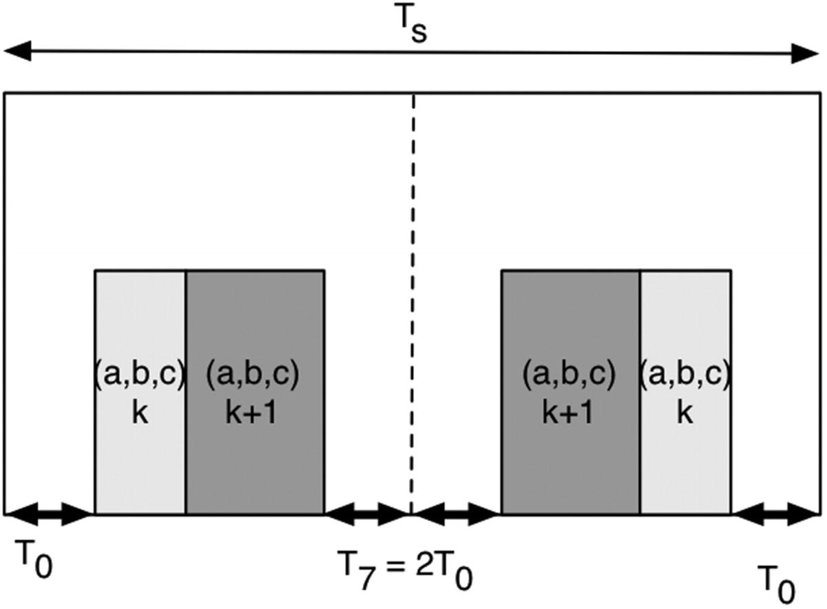
Pulse period segments. Each pulse period T s is divided into seven segments so that the two switching patterns k and k + 1 are applied symmetrically.


$$displaystyle egin{aligned} T_0 = frac{1}{4}left(T_s - (T_k + T_{k+1})
ight) end{aligned} $$
(9.22)
The implementation of the pulse segments is slightly different for the even and odd sectors in Figure 9.4. Both are symmetric about the midpoint of the pulse as described, but we reverse the implementation of patterns k and k + 1. This is shown for the resulting voltages u in the following equations. We use the first in even sectors and the second in odd sectors.

$$displaystyle egin{aligned} left[ egin{array}{lllllll} u_0&u_k&u_{k+1}&u_7&u_{k+1}&u_k&u_0 end{array} 
ight] end{aligned} $$
(9.23)
and

$$displaystyle egin{aligned} left[ egin{array}{lllllll} u_0&u_{k+1}&u_k&u_7&u_k&u_{k+1}&u_0 end{array} 
ight] end{aligned} $$
(9.24)

Using the different patterns for odd and even vectors minimizes the number of commutations per cycle.

We determine the sector from the angle Θ formed by the commanded voltages u α and u β:

$$displaystyle egin{aligned} varTheta = mathrm{atan}frac{u_eta}{u_alpha} end{aligned} $$
(9.25)

The pulsewidth modulation routine, SVPWM, does not actually perform an arctangent. Rather, it looks at the unit u α and u β vectors and determines first their quadrant and then their sector without any need for trigonometric operations.

The first section of SVPWM implements the timing for the pulses. Just as in the previous recipe for the controller, the function uses its data structure as memory – the updated structure is passed back as an output. This is an alternative to persistent variables.

SVPWM.m

../images/335353_2_En_9_Chapter/335353_2_En_9_Fige_HTML.gif

The pulsewidth vectors are computed in the subfunction SVPW. We first compute the quadrant and then the sector without using any trigonometric functions. This is done using simple if/else statements and a switch statement. Note that the modulation index k is simply designated k and k + 1 is designated kP1. We then compute the times for the two space vectors that bound the sector. We then assemble the seven subperiods.

../images/335353_2_En_9_Chapter/335353_2_En_9_Figf_HTML.gif

../images/335353_2_En_9_Chapter/335353_2_En_9_Figg_HTML.gif

../images/335353_2_En_9_Chapter/335353_2_En_9_Figh_HTML.gif

The built-in demo is fairly complex so it is in a separate subfunction. We simply specify an example input u using trigonometric functions.

../images/335353_2_En_9_Chapter/335353_2_En_9_Figi_HTML.gif

Figure 9.6 shows the state vector pulsewidth modulation from the built-in demo. There are three pulses in the plot, each 0.001 seconds long. Each pulse period has seven subperiods.
../images/335353_2_En_9_Chapter/335353_2_En_9_Fig6_HTML.jpg
Figure 9.6

The desired voltage vector and the Space Vector Modulation pulses and pulsewidth. The bottom plot shows the pulse periods. Note that the pulse sequences are symmetric within each pulse period.

The function SwitchToVoltage converts switch states to voltages. It assumes instantaneous switching and no switch dynamics.

SwitchToVoltage.m

../images/335353_2_En_9_Chapter/335353_2_En_9_Figj_HTML.gif

9.4 Simulating the Controlled Motor

Problem

We want to simulate the motor with torque control using Space Vector Modulation.

Solution

Write a script to simulate the motor with the controller. We include options for closed loop control and balanced three-phase voltage inputs.

How It Works

The header for the script, PMMachineDemo, is shown in the following listing. The control flags bypassPWM and torqueControlOn are described as well as the two periods implemented, one for the simulation and a longer period for the control.

PMMachineDemo.m

../images/335353_2_En_9_Chapter/335353_2_En_9_Figk_HTML.gif

The body of the script follows. Three different data structures are initialized from their corresponding functions as described in the previous recipes, that is, from SVPWM, TorqueControl, and RHSPMMachine. Note that we are only simulating the motor for a small fraction of a second, 0.05 seconds, and the time step is just 1e-6 seconds. The controller time step is set to 100 times the simulation time step.

../images/335353_2_En_9_Chapter/335353_2_En_9_Figl_HTML.gif

../images/335353_2_En_9_Chapter/335353_2_En_9_Figm_HTML.gif

../images/335353_2_En_9_Chapter/335353_2_En_9_Fign_HTML.gif

We turn off torque control to test the motor simulation with the results shown in Figure 9.7. The two plots show the torque speed curves. The first is with direct three-phase excitation, that is, bypassing the pulsewidth modulation, by setting bypassPWM to false. Directly controlling the phase voltages this way, while creating the smoothest response, would require linear amplifiers which are less efficient than switches. This would make the motor much less efficient overall and would generate unwanted heat. The second plot is with Space Vector Pulsewidth Modulation. The plots are nearly identical, indicating that the pulsewidth modulation is working.
../images/335353_2_En_9_Chapter/335353_2_En_9_Fig7_HTML.jpg
Figure 9.7

Torque speed curves for a balanced three-phase voltage excitation and a load torque of 1.0 Nm. The left figure shows the curve for the direct three-phase input, and the right shows the curve for the Space Vector Pulsewidth Modulation input. They are nearly identical.

We now turn on torque control, via the torqueControlOn flag, and get the results shown in Figure 9.8. The overshoot is typical for torque control. Note that the load torque is set equal to the torque set point of 1 Nm. There is limit cycling near the end point.
../images/335353_2_En_9_Chapter/335353_2_En_9_Fig8_HTML.jpg
Figure 9.8

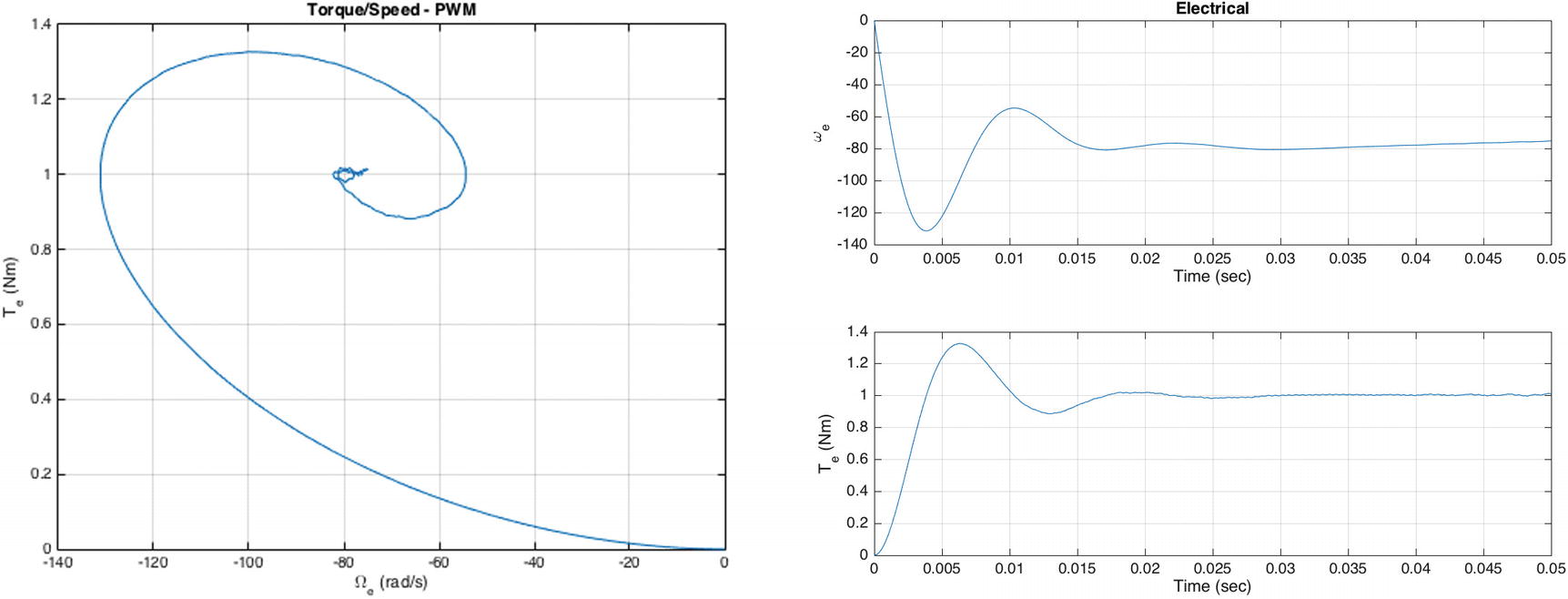
PI torque control of the motor.

The pulsewidths and resulting coil currents are shown in Figure 9.9. A zoomed view of the end of the pulsewidth plot with shading added to alternate pulsewidths is in Figure 9.10. This makes it easier to see the segments of the pulsewidths and verify that they are symmetric.
../images/335353_2_En_9_Chapter/335353_2_En_9_Fig9_HTML.jpg
Figure 9.9

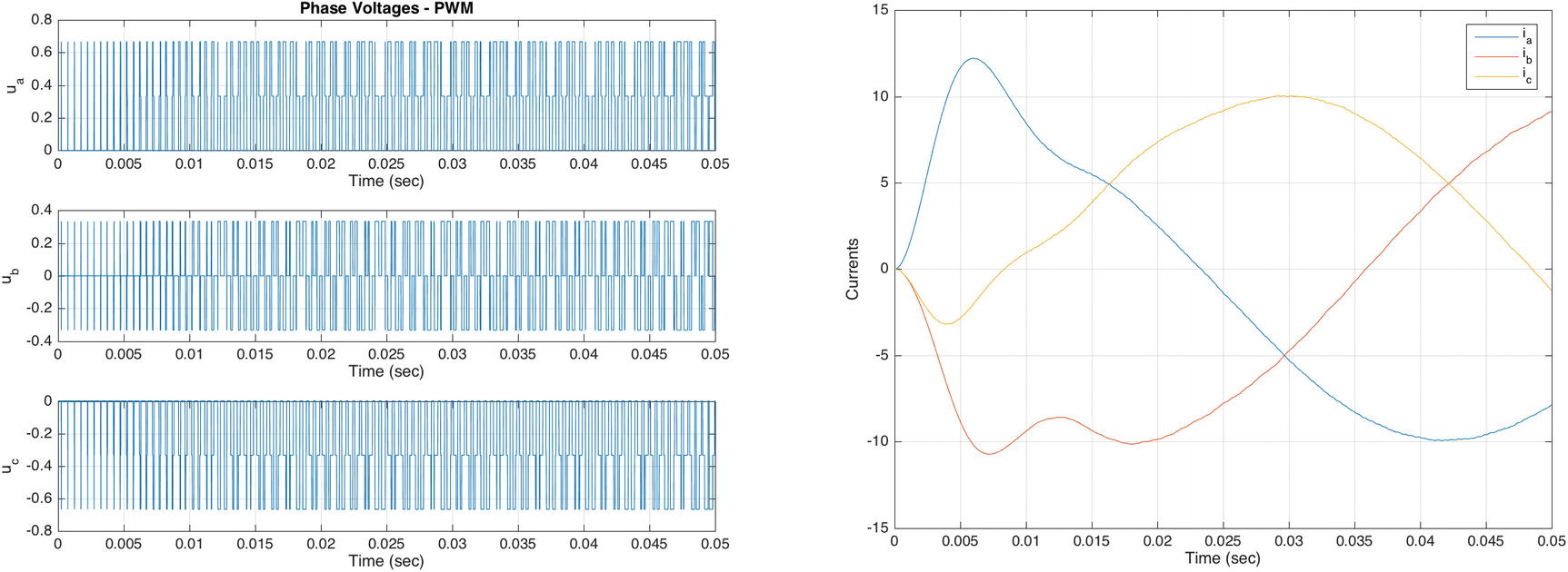
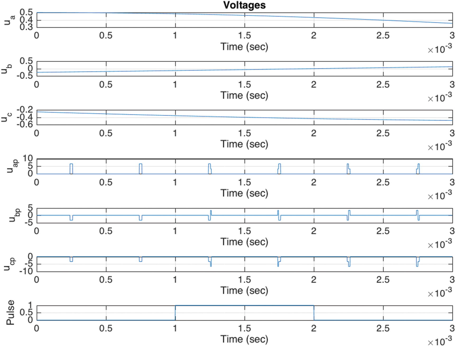
Voltage pulsewidths and resulting currents for PI torque control.

../images/335353_2_En_9_Chapter/335353_2_En_9_Fig10_HTML.jpg
Figure 9.10

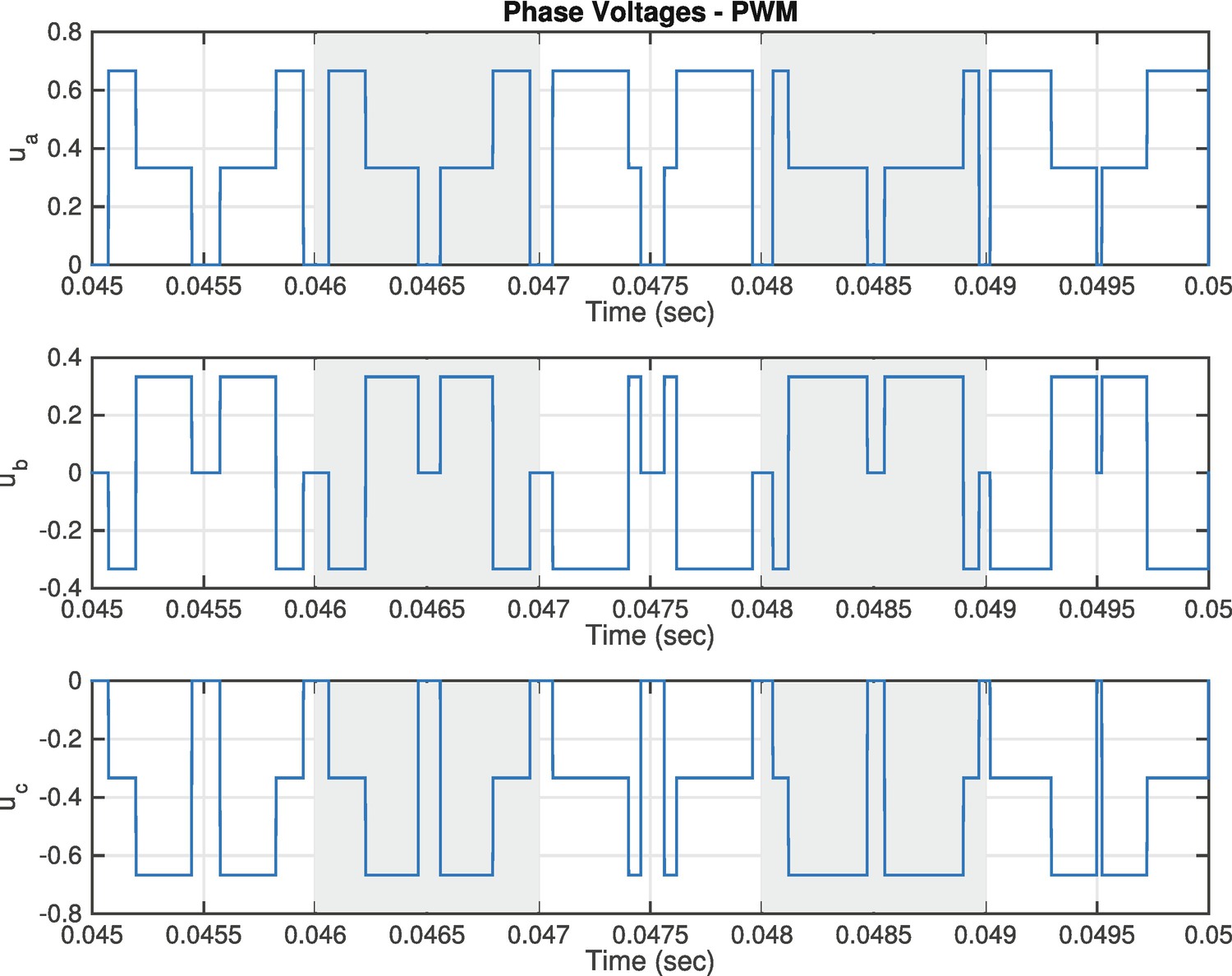
Pulsewidths with shading.

The code which adds the shading uses fill with transparency via the alpha parameter. In this case, we hard-code the function to show the last five pulsewidths, but this could be generalized to a time window, or to shade the entire plot. We did take the time to add an input for the pulsewidth length, so that this could be changed in the main script and the function would still work. Note that we reorder the axes children as the last step, to keep the shading from obscuring the plot lines.

AddFillToPWM.m

../images/335353_2_En_9_Chapter/335353_2_En_9_Figo_HTML.gif

9.5 Summary

This chapter has demonstrated how to write the dynamics and implement a field-oriented control law for a three-phase motor. We use a proportional-integral controller with Space Vector Pulsewidth Modulation to drive the six switches. This produces a low-cost controller for a motor. Table 9.2 lists the code developed in the chapter.
Table 9.2

Chapter Code Listing

File

Description

AddFillToPWM

Add shading to the motor pulsewidth plot

ClarkeTransformationMatrix

Clarke transformation matrix

ParkTransformationMatrix

Park transformation matrix

PMMachineDemo

Permanent magnet motor demonstration

RHSPMMachine

Right-hand side of a permanent magnet brushless three-phase electrical machine

SVPWM

Implements Space Vector Pulsewidth Modulation

SwitchToVoltage

Converts switch states to voltages

TorqueControl

Proportional-integral torque controller

..................Content has been hidden....................

You can't read the all page of ebook, please click here login for view all page.
Reset
18.191.216.163