
The XLOOKUP function was released in 2020 to provide a superior lookup function to others that have existed in Excel for years.
This function is the new kid on the block of lookup functions. It gains more fans every week as Excel users discover XLOOKUP and the simplicity it provides in looking up and returning values.
This function is only available for users of Excel 2021 (Windows and Mac), Excel for Microsoft 365 (Windows and Mac), and Excel for the Web. It is a fine representation of how we work in modern Excel.
In this chapter, we will begin with the basics of XLOOKUP and use the function to accomplish some typical lookup tasks. We then progress through numerous examples that demonstrate the power of this function.
xlookup.xlsx
Introduction to XLOOKUP
Availability : Excel 2021, Excel for Microsoft 365, Excel for the Web, Excel 2021 for Mac, Excel for Microsoft 365 for Mac
The XLOOKUP function combines a blend of the key attributes of the INDEX and MATCH functions into one function. It is a brilliant function with some special abilities.
Its modest definition is that it looks for a value, within a range or array, and returns the corresponding item from a second range or array. However, you soon realize it goes a little beyond this scope.
It defaults to an exact match. This is the most common match type yet is not the default with the older VLOOKUP and MATCH functions.
It contains a built-in if not found argument. No requirement for a function such as IFERROR or IFNA to handle unmatched values.
It can return ranges as well as values. VLOOKUP cannot do this. This complements the dynamic array engine wonderfully.
It is a robust lookup function. It can look vertically or horizontally, left or right, and does not require the values of its lookup array to be in any specific order.
It can look for a value from first to last or last to first.
The XLOOKUP function is especially well equipped at performing lookups on data in tables, returning ranges and working with dynamic arrays. These are key qualities of XLOOKUP.
Lookup functions such as INDEX, VLOOKUP, HLOOKUP, and OFFSET request index numbers for their row and column arguments. This makes them great for relative references and more flexible. XLOOKUP works with explicit references to the range or table element to be used for its lookup and return arrays. XLOOKUP is a perfect match for use with structured data in tables. They go together like mint and chocolate. A dream team.
Lookup value: The value you are looking for
Lookup array: The range or array to look within
Return array: The range or array to return from
[If not found]: The value to return if a match is not found
- [Match mode]: The number –1, 0, 1, or 2 that defines the match type
0 is entered to specify an exact match. This is the most used match type and the default option.
–1 is entered to return the position of the exact match or the next smaller value to the lookup value, if the lookup value is not found.
1 is entered to return the position of the exact match or the next larger value to the lookup value, if the lookup value is not found.
2 is entered to specify a wildcard character match. The asterisk (*), question mark (?), and tilde (~) wildcard characters can be used for partial matches.
- [Search mode]: The number 1, –1, 2, or –2 that defines the type of search to perform
1 is entered to specify a search from first to last (top to bottom). This is the default search mode.
–1 is entered to reverse the search and search from last to first (bottom to top).
2 is entered to specify a binary search from first to last. Performing this type of search requires the lookup array to be sorted in ascending order.
–2 is entered to specify a binary search from last to first. The lookup array needs to be sorted in descending order for this type of search.
XLOOKUP for an Exact Match
XLOOKUP makes exact match lookups very simple and very durable, especially when used with data formatted as a table.

Table of product data
All data sheets in the example [xlookup.xlsx] file have been hidden.

XLOOKUP returning the product name for each ID value
This is very simple. There is no requirement to enter a column index number as requested by VLOOKUP or to nest a MATCH function as commonly used with INDEX.
Specifying table columns instead of ranges that lack meaning, such as column 5 or range E2:E14, makes it even better. It is faster to enter the formula too – less clicking with a mouse to select ranges, typing in meaningful references instead.
The XLOOKUP function has a built-in argument to specify an if not found value to return instead of the #N/A error. This is optional and is often not required.

If not found argument returning a value instead of #N/A
Because the XLOOKUP function uses distinct lookup and return arrays (VLOOKUP looks in and returns from the same table array), the lookup array and return array can be in any order within the lookup table.

Returning the category name for each product ID
The value in cell C4 has been changed back from 152 to 151 to return a matching value.
XLOOKUP to Look Up a Value in Ranges
The different match modes of XLOOKUP can be split into three different types of lookups – exact matches, range lookups, and wildcard lookups.

The different match modes of XLOOKUP
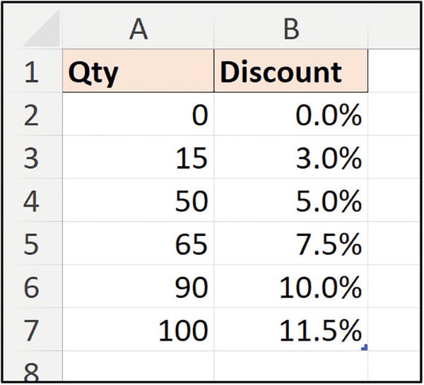
Table of quantity ranges and discounts

Looking up a value in ranges with XLOOKUP
Although the ranges of [Qty] values in [tblDiscounts] are in ascending order, and it is great that they are, the XLOOKUP function returns the correct discount regardless of the order of the ranges.
This provides a more robust range lookup formula than offered by the older VLOOKUP and MATCH functions. They required the range values to be in order.
XLOOKUP with Wildcards
The XLOOKUP function can handle the use of wildcard characters such as the asterisk (*) and question mark (?) in the lookup value, but this needs to be specified as the match mode.

Table containing cities and targets
From another range, we have a column that contains city names only, for example, “Lisbon,” and we need to look up the city in the [tblTargets] table and return the [Target] value.
We need to perform a partial match on the city name, as there is not an exact match between the two column values. For this, we can perform a wildcard search.
* (Asterisk): Represents any number of characters. For example, New* would match with Newport, Newcastle, New York, and New Zealand.
? (Question mark): Represents a single character. For example, L????n would match with both London and Lisbon.
~ (Tilde): Used to treat a wildcard character as a text character. For example, *don would match any text that ends in the characters don, but ~*don will look for an exact match of *don, treating the asterisk as its character and not a wildcard.
For the lookup value, the city name in column C is combined with the asterisk wildcard character. This creates a lookup value that begins with the value in column C but can have any text after that.

XLOOKUP function using wildcard characters in the lookup value
XLOOKUP for the Last Match
One of the key developments with the XLOOKUP function compared to some other lookup functions is its ability to search its lookup array from last to first in addition to the standard first to last.
Figure 12-10 shows a table named [tblCourses] that contains a list of training courses that were conducted recently. The courses are ordered by the date that they were delivered.

Table of recently delivered training courses

Returning the last matching value in a list
An empty string “” is specified for the if not found argument. The XLOOKUP formula in cell F3 returns “No courses booked” if there is no matching value, so it is not necessary to provide a meaningful if not found response again. We just want to hide the #N/A error, and an empty string is ideal for that task.
Multiple Column XLOOKUP
With XLOOKUP, it is simple to create lookup formulas that return values or ranges where the values in multiple columns must match. These formulas are sometimes referred to as multi-criteria lookup formulas.

Table containing prices by membership type and location
The values in cells B2 (membership) and C2 (location) are combined into one value using the ampersand (&). The same technique is applied to the columns required for the lookup array – [Membership] and [Location].

Multiple column XLOOKUP formula
Two-Way Lookup with XLOOKUP
What is better than XLOOKUP? Two XLOOKUPs. And with two XLOOKUP functions, we can create a two-way lookup.
This two-way lookup formula uses an XLOOKUP to return the matching value from an array returned by an accompanying XLOOKUP function.

Accommodation prices for the two-way lookup

Two-way XLOOKUP formula
The second XLOOKUP is finding the matching column, while the first finds the matching row.
The second XLOOKUP function is used as the return array for the first XLOOKUP. The second XLOOKUP returns the array of values corresponding to the value stated in the [Location] column.
The first XLOOKUP then returns the corresponding value in this array for the value stated in the [Accommodation] column.
It does not matter which order the two XLOOKUP functions are used; however, I have written them in order of row and then column to match R1C1 notation.
Three-Way Lookup
We can combine the techniques of the last two examples to create what some refer to as a three-way lookup.
The second XLOOKUP function is returning the array of values for the matching column like we saw in the two-way lookup example. It is matching the day of week value in cell C2 against the range of values in C4:I4.
The first XLOOKUP then returns the corresponding value in that array for the matching row. The room type and board conditions are met by combining the values from A2 and B2 and A5:A10 and B5:B10. This creates a merged lookup value and lookup array.

Three-way lookup with XLOOKUP
Three-Way Lookup with Mixed Match Modes
Taking the previous example further, the XLOOKUP functions can use different match modes. In Figure 12-17, we have a range containing different room rates that are dependent upon the room type, board, and the time of the year. This range is on a sheet named [Room Rates].
In range C1:F1 are ranges of dates beginning from 10th March 2021. The price of a room changes at different times of the year.

Room rates over different date periods

Three-way lookup including date ranges
Returning Multiple Values with XLOOKUP
In the last few examples demonstrating two- and three-way lookups, we have seen that an XLOOKUP function can return an array of values for a matching value in a row or column. In each of those examples, the array was passed to another XLOOKUP to return a single matching value.
This array returned by XLOOKUP can, of course, be passed to other Excel functions for use or to the grid itself.
In this example, the values are returned to the grid to be displayed. A defined name could be made for this spill range of values and then used as the data source for a chart like the example at the end of Chapter 10.

Returning multiple values with XLOOKUP
In this example, the values are returned in the same order as displayed in the lookup array. This works in this scenario, and because the labels in range C1:G1 are month names, the order is unlikely to change.
Another XLOOKUP is added to the formula to match the values in range C1:G1 to the header labels in range C4:G4. This returns an array with the values in the order that they are matched, as opposed to inferring that the order of the two ranges is the same.

Returning multiple values in a different order with XLOOKUP
This also provides a more robust formula – one that is unaffected by users changing the order of the values in the lookup array or the lookup values in range C1:G1.
The formula returns a spill range of the resulting values. This is efficient, as it is only one formula returning multiple results.
Instead of returning the values to the grid, they can be returned to another function for use, such as an aggregation function like SUM.

Summing the array of values returned by XLOOKUP
XLOOKUP with SUMIFS for a Dynamic Sum Range
The XLOOKUP function can be used with SUMIFS to provide a dynamic column for the sum range. The sum range column can be specified by a cell value. This technique works equally well with AVERAGEIFS, COUNTIFS, etc.

XLOOKUP with the SUMIFS function
To keep the formula as meaningful as possible, XLOOKUP is told to check the entire header row of the [tblExpenses] table, even though only the location columns need checking.
Plus, by referencing the entire header row, if a new location/column is added, the formula continues to work.
XLOOKUP with Other Excel Features
We will conclude the chapter by going beyond the grid and use XLOOKUP with other Excel features. We start with an example of using XLOOKUP to create dependent drop-down lists. This example demonstrates a special technique of using the spill reference appended to the end of a function.
Dependent Drop-Down List with XLOOKUP
A dependent drop-down list is when the items in a list are dependent upon the item selected from a previous list. XLOOKUP provides a neat way for us to set up these dependent drop-down lists in Excel.

Spill ranges to be used for dependent drop-down list
The FILTER function is covered in detail in Chapter 13. This is a brilliant function.
We will create a dependent drop-down list so that when a user picks a country from the list, the second list only displays the cities for that selected country.
We want to use the XLOOKUP function to work with the spill ranges returned by the FILTER function. There may be additional cities added or cities removed in the future. By accessing the spill ranges, the drop-down lists would automatically update.
Also, by working directly with the spill ranges, we can avoid the additional blank cells that would appear if we selected the ranges manually. In this example, there are fewer cities in “Spain” in our data than for other countries.

Drop-down list of country names
- 1.
Select range C2:C4.
- 2.
Click Data ➤ Data Validation.
- 3.
Click the Allow list and click List. Enter the following formula into the Source box (Figure 12-25). Click OK.
The formula searches for the country specified in the first drop-down along range Lists!$D$1:$G$1. An absolute reference is used as the Data Validation rule is applied to multiple cells in this example.

XLOOKUP formula in a Data Validation rule
A name could have been defined for the XLOOKUP formula and then referenced in the Data Validation rule. We have covered this technique previously in this book. It is useful to aid the management of formulas.

Dependent drop-down list of cities
This Data Validation rule can be applied to as many cells in columns B and C as required. To simplify the example, the rule is applied to rows 2:4 only. However, we could easily have selected a larger range to apply the Data Validation rules to.
Return a Range for a Chart
The XLOOKUP function can be used to return a range like we saw with the INDEX function in Chapter 11. While INDEX is excellent at relative references and working with index values such as column numbers, XLOOKUP is better for explicit column references and is more succinct for ranges between text values.

Sales for all months with input cells to specify a range
We want to create a line chart showing the sales for the product specified in cell B2 and for the date range specified by the months in cells C2 and D2.
To do this, we will create two different XLOOKUP formulas: one for the month names to be used in the chart’s X axis and another for the sales values to be used for the chart data series.
Names will be defined for each of the two XLOOKUP formulas and then used for the two elements of the line chart.
Let’s enter the two formulas on the worksheet first. This is not necessary; however, it is good practice, as it provides an opportunity to check that the formulas work correctly, before proceeding to define the names and the subsequent chart steps.

XLOOKUP formulas entered on the worksheet
- 1.
Copy the text for the formula returning the month names.
- 2.
Click Formulas ➤ Define Name.
- 3.
Type “MonthLabels” for the Name of the formula.
- 4.
Paste the formula into the Refers to box (Figure 12-29). Click OK.

Defining a name for the chart labels
- 5.
Repeat these steps to define a name for the formula that returns the sales values. Name it “MonthValues.”
The sheet name is added automatically by Excel to each of the references in the named formulas.
- 1.
Click Insert ➤ Insert Line or Area Chart ➤ Line to insert a blank line chart.
- 2.
With the chart selected, click Chart Design ➤ Select Data. This opens the Select Data Source window (Figure 12-32).
- 3.
Click the Add button in the Legend Entries (Series) area of the window.
- 4.
Click in the Series name box and click cell B2 containing the name of the selected product (Figure 12-30).
- 5.
Remove the text in the Series values box, click a cell on the worksheet to enter the sheet name quickly, delete the cell reference, and type “MonthValues”. Click OK.

Editing the chart data series

Editing the chart labels
- 6.
Click the Edit button in the Horizontal (Category) Axis Labels area of the window.
- 7.
Remove the text in the Axis label range box, click a cell on the worksheet to enter the sheet name quickly, delete the cell reference, and type “MonthLabels” (Figure 12-31). Click OK.
Instead of typing the name, you can also press F3 to open the Paste Name window, select the name, and click OK.

Completed data source for the chart

Completed chart from a specified range
Summary
In this chapter, we learned the new XLOOKUP function – a powerful and robust function, built for modern Excel, with its ability to work with tables, arrays, and dynamic ranges effortlessly.
This was supported by practical examples, including performing multi-criteria lookups and returning dynamic ranges for dependent lists and chart ranges. We also covered the developments that were made to improve on its predecessors VLOOKUP and HLOOKUP.
In the next chapter, we will dive into the FILTER function in Excel – another fantastic function that makes you wonder how we managed without it.
FILTER is another lookup function, one that returns all matching values. We will see numerous examples of its use to showcase its benefits and see how it can be applied in “real-world” scenarios.