Data Representation

The first choice of technology we need to make is how to represent the data. Some of the choices are:

• Protocol Buffers (https://developers.google.com/protocol-buffers)

• Apache Thrift (https://thrift.apache.org/)

• JSON (https://www.json.org/json-en.html)

• XML (https://developer.mozilla.org/en-US/docs/Web/XML/XML_introduction)

• CSV (https://en.wikipedia.org/wiki/Comma-separated_values)

In this implementation we go with Protocol Buffers mostly because of the ease of specifying a schema and then subsequently serializing and deserializing them.

For the file format we use serialized protocol buffers that are then UUencoded and written as a single line per record and then bzipped up for compression. This is just for convenience so that we can parse the files easily without having dependencies on too many libraries.

Your company might instead store data in a data warehouse that is accessible by SQL for example.

Protocol buffers are generally easier to parse and handle than raw data. In our implementation we will parse the wikipedia XML into protocol buffers for easier handling using xml2proto.py. You can see from the code that XML parsing is a complicated affair, whereas protocol buffer parsing is as simple as calling a method called ParseFromString and all the data is then subsequently available as a convenient Python object.

As of June 2022, the Wikipedia dump is about 20GB in size and it takes about 10 minutes to convert to protocol buffer format. Please follow the steps described in the README in the GitHub repo for the most up to date steps to run the programs.

In the proto directory, take a look at some of the protocol messages defined. This for example is how we might store the text from a wikipedia page.

// Generic text document.
message TextDocument {
  // Primary entity, in wikipedia it is the title.
  string primary = 1;
  // Secondary entity, in wikipedia it is other titles.
  repeated string secondary = 2;
  // Raw body tokens.
  repeated string tokens = 3;
  // URL. Only visible documents have urls, some e.g. redirect shouldn't.
  string url = 4;
}

The types supported and the schema definitions can be found on the protocol buffer documentation page. This schema is converted into code using the proctocol buffer compiler. The protocol buffer compiler’s job is to convert the schema into code that you can call in different languages, which in our case is to access the data in python. The installation of the protocol buffer compiler depends on the platform and instructions to install them can be found in the Protocol buffer documentation.

Each time you change the schema you will have to use the protocol buffer compiler to get a new version of the protocol buffer code. This step can easily be automated by using a build system like Bazel but this is out of scope for this book. For the purposes of this book we will simply generate the protocol buffer code once and check it into the repository for simplicity.

Following the directions on the github README, download a copy of Wikipedia, then run xml2proto.py to convert it to a procol buffer format. Optionally use codex.py to see what the protocol buffer format looks like. These steps took 10 minutes on a Windows workstation using Windows Subsystem for Linux. The XML parser used doesn’t parallelize very well so this step is fundamentally serial. We’ll discuss next how we would distribute the work in parallel either among multiple cores locally or on a cluster.

Big Data Frameworks

The next technology choice we are going to make is the technology to process data at scale on multiple machines.

Some options are:

• Apache Spark (https://spark.apache.org/)

• Apache Beam (https://beam.apache.org/)

• Apache Flink (https://flink.apache.org/)

In this implementation we chose Apache Spark in Python, or PySpark. The README in the repository shows how to install a copy of PySpark locally using pip install.

The first step that is implemented in pyspark is the step called tokenization and url normalization. The code is in tokenize_wiki_pyspark.py but we won’t go over it in the book because a lot of the processing is simply distributed natural language parsing and writing out the data into procol buffer format. We will instead talk in detail about the second step, which is to make a dictionary of tokens (the words in the article) and have some statistics about the word counts. However, we will run it just to see what the spark usage experience looks like. Spark programs are run using the program spark-submit as follows:

bin/spark-submit
--master=local[4]
--conf="spark.files.ignoreCorruptFiles=true"
tokenize_wiki_pyspark.py
--input_file=data/enwiki-latest-parsed --output_file=data/enwiki-latest-tokenized

Running the Spark submit script allows you to execute the controller program, in this case tokenize_wiki_pyspark.py on a local machine like we have in the command line – note that the line local[4] means use up to four cores. The same command can be used to submit the job to a YARN cluster for running on hundreds of machines, but for the purposes of trying out PySpark, a decent enough workstation should be able to process all the data in minutes. This tokenization program converts from a source specific format, in this case a Wikipedia protocol buffer, into a more generic text document used for natural language processing. In general it’s a good idea to use a generic format that all your different sources of data can be converted into because it simplifies the data processing downstream. The data conversion can be done from each corpus into a standard format that is handled uniformly by all the later programs in the pipeline.

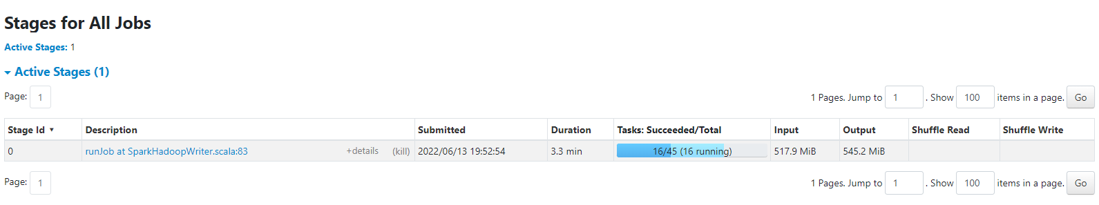
Figure 8-1. Spark UI

After submitting the job you can then navigating to the Spark UI (as shown in Figure 8-1 on your local machine at http://localhost:4040/stages/ you should see the job executing in parallel using up all the cores in your machine. You might want to play with the local[4] parameter, if you use local[*] it will use up all the free cores on your machine. If you have access to a cluster, you can also point to the appropriate cluster url.

Cluster Frameworks

The nice thing about writing a Spark program is that your program can scale from a single machine with multiple cores to a cluster with many machines with thousands of cores. The full list of cluster types can be found in the Spark Submit Documentation.

Spark can run on the following cluster types:

• Spark Standalone Cluster (https://spark.apache.org/docs/latest/spark-standalone.html)

• Mesos Cluster (https://mesos.apache.org/)

• YARN Cluster (https://hadoop.apache.org/docs/stable/hadoop-yarn/hadoop-yarn-site/YARN.html)

• Kubernetes Cluster (https://kubernetes.io/)

Depending on what kind of cluster your company or institution has set up most of the time it is just a matter of pointing to the correct URL in order to submit the job.

Many companies such as DataBricks and Google also have fully mananaged Spark solutions that allow you to setup a Spark cluster with very little effort.

PySpark Example

Counting words turns out to be a really powerful tool in information retrieval as we can use some handy tricks like TF-IDF or term frequency, inverse document frequency which is simply the count of words in the documents divided by the number of document the word has occured in. This is represented as:

For example the word “the” is frequent and one might think it is an important word, but by dividing by the document frequency, the world “the” is therefore less special and drops in importance. This trick is quite handy in simple natural language processing to get a better than random weighting of word importance.

Therefore, the next thing we are going to do is run make_dictionary.py. As the name implies this program simply counts the words and documents and makes a dictionary with the number of times a word has occured.

There are some concepts to cover in order to properly grok how Spark helps one process data in a distributed manner. The entry point of most Spark programs is the Spark Context. It is a Python object that is created on the controller. The controller is the central program that launches workers which actually process the data. The workers can be run locally on a single machine as a process or on many machines on the cloud as separate workers.

The Spark Context can be used to create resilient distributed data, or RDDs. These are references to data streams that can be manipulated on the controller and processing on the RDD can be farmed out to all the workers. The Spark Context allows one to load up data files stored on a distributed file system like Hadoop distributed file system (HDFS) or cloud buckets. By calling the Spark Context’s textFile method we are returned a handle to an RDD. A stateless function can then be applied or mapped on the RDD to transform it from one RDD to another by repeatedly applying the function to the contents of the RDD.

For example, this program fragment loads a text file and converts all lines to lowercase by running an anonymous lambda function that converts single lines to lowercase.

def lower_rdd(input_file: str,
              output_file: str):
  """Takes a text file and converts it to lowercase.."""
  sc = SparkContext()
  input_rdd = sc.textFile(input_file)
  input_rdd.map(lambda line: line.lower()).saveAsTextFile(output_file)

In a single machine implementation, we would simply load up each Wikipedia article, keep a running dictionary in RAM and simply count each token and add one to the token count in the dictionary. A token is an atomic element of how a document is broken up into pieces. In regular English it would be a word, but in the case of Wikipedia documents there are other entities such as the document references themselves that need to be kept track of separately, so we call the breaking up into pieces tokenization and the atomic elements tokens. The single machine implementation would take a while to go through the thousands of documents on Wikipedia which is why we use a distributed processing framework like Spark. In the Spark paradigm, computation is broken up into maps, where a function is applied statelessly on each document in parallel. There is also reduce, where the outputs of separate maps are joined together.

For example suppose we had a list of word counts and we wanted to sum up the values of words that occurred in different documents, then the input to the reducer would be something like:

• (apple, 10)

• (orange, 20)

• (apple, 7)

Then we would call the Spark function reduceByKey(lambda a, b: a+ b) which would add all the values with the same key together which would return

• (orange, 20)

• (apple, 17)

If you look at the code in make_dictionary.py the map phase is where we take a document as input and then break it into tuples of (token, 1). In the reduce phase, the map outputs are joined by the key, which in this case is the token itself, and the reduce function is simply to sum up all the counts of tokens. Note that the reduce function assumes that the reduction is associative, that is $(a+b+c)=(a+b)+c=a+(b+c)$ which allows the Spark framework to sum up some parts of the token dictionary in memory on the map phase (in some frameworks this is called the combine step, where you run part of the reduction on the output of the map phase on the mapper machine), and then sum them up over several passes on the reduce phase. As an optimization, we use the Spark function mapPartitions. Map runs the provided function once per line (for which we have encoded an entire Wikipedia document as a protocol buffer, UUencoded as a single text line), whereas mapPartitions runs it over an entire partition which is many documents, usually 64MB of them. This optimization lets us construct a small Python dictionary over the entire partition so that there are many fewer less token-count pairs to reduce. This saves on network bandwidth so the mapper has less data to send to the reducer, and is a good tip in general for these data processing pipelines to reduce network bandwidth which is generally the most time consuming part of data processing compared to computation.

Here we show a complete Spark program that reads in documents in the protocol buffer format of TextDocument shown above and then counts how often the words, or tokens occur in the entire corpus. The file in the github repo is make_dictionary.py. It is presented slightly differently from the repo file in that it is broken into three chunks for readability and the order of the main and subroutines have been swapped for clarity. In the book we present first the dependencies and flags, then the main body then the functions being called by the main body so that the purpose of the functions are clearer.

Firstly, we have the dependencies. The main ones are the protocol buffer representing the text document of the Wikipedia article as discussed earlier. This is the input we are expecting. For the output we have the TokenDictionary protocol buffer which mainly counts the occurrences of words in the article. We will use the co-occurrences of words to form a similarity graph of articles that we can then use as the basis of a warm start recommender system. We also have dependencies on pyspark, the data processing framework we are using to process the data as well as a flag library that handles the options of our program. The absl flags library is pretty handy in parsing and explaining the purposes of command line flags and also retrieving the set values of flags easily.

#!/usr/bin/env python
# -*- coding: utf-8 -*-
#
#

"""
  This reads a doc.pb.b64.bz2 file and generates a dictionary.
"""
import base64
import bz2
import nlp_pb2 as nlp_pb
import re
from absl import app
from absl import flags
from pyspark import SparkContext
from token_dictionary import TokenDictionary

FLAGS = flags.FLAGS
flags.DEFINE_string("input_file", None, "Input doc.pb.b64.bz2 file.")
flags.DEFINE_string("title_output", None,
                    "The title dictionary output file.")
flags.DEFINE_string("token_output", None,
                    "The token dictionary output file.")
flags.DEFINE_integer("min_token_frequency", 20,
                     "Minimum token frequency")
flags.DEFINE_integer("max_token_dictionary_size", 500000,
                     "Maximum size of the token dictionary.")
flags.DEFINE_integer("max_title_dictionary_size", 500000,
                     "Maximum size of the title dictionary.")
flags.DEFINE_integer("min_title_frequency", 5,
                     "Titles must occur this often.")

# Required flag.
flags.mark_flag_as_required("input_file")
flags.mark_flag_as_required("token_output")
flags.mark_flag_as_required("title_output")

Next, we have the main body of the program which is where all the subroutines are called. We first create a Spark Context which is the entry point into the Spark data processing system and we call it’s method textFile to read in the bzipped Wikipedia articles. Please read the README.md on the repo as to how it was generated. Next, we parse the text document and send the RDD to two different processing pipelines, one to make a dictionary for the body of the article and another to make a dictionary of the titles. One could choose to make a single unified dictionary for both, but having them separate allows us to create a content based recommender using the token dictionary and an article to article recommender using the title dictionary as titles are identifiers for the Wikipedia article.

def main(argv):
  """Main function."""
  del argv  # Unused.
  sc = SparkContext()
  input_rdd = sc.textFile(FLAGS.input_file)
  text_doc = parse_document(input_rdd)
  make_token_dictionary(
    text_doc,
    FLAGS.token_output,
    FLAGS.min_token_frequency,
    FLAGS.max_token_dictionary_size
  )
  make_title_dictionary(
    text_doc,
    FLAGS.title_output,
    FLAGS.min_title_frequency,
    FLAGS.max_title_dictionary_size
  )


if __name__ == "__main__":
    app.run(main)

Finally we have the subroutines called by the main function all decomposed into smaller subroutines for counting the tokens in the article body and the titles.

def update_dict_term(term, dictionary):
    """Updates a dictionary with a term."""
    if term in dictionary:
        x = dictionary[term]
    else:
        x = nlp_pb.TokenStat()
        x.token = term
        dictionary[term] = x
    x.frequency += 1


def update_dict_doc(term, dictionary):
    """Updates a dictionary with the doc frequency."""
    dictionary[term].doc_frequency += 1


def count_titles(doc, title_dict):
    """Counts the titles."""
    # Handle the titles.
    all_titles = [doc.primary]
    all_titles.extend(doc.secondary)
    for title in all_titles:
        update_dict_term(title, title_dict)
    title_set = set(all_titles)
    for title in title_set:
        update_dict_doc(title, title_dict)


def count_tokens(doc, token_dict):
    """Counts the tokens."""
    # Handle the tokens.
    for term in doc.tokens:
        update_dict_term(term, token_dict)
    term_set = set(doc.tokens)
    for term in term_set:
        update_dict_doc(term, token_dict)


def parse_document(rdd):
    """Parses documents."""
    def parser(x):
        result = nlp_pb.TextDocument()
        try:
            result.ParseFromString(x)
        except google.protobuf.message.DecodeError:
            result = None
        return result
    output = rdd.map(base64.b64decode)
        .map(parser)
        .filter(lambda x: x is not None)
    return output


def process_partition_for_tokens(doc_iterator):
    """Processes a document partition for tokens."""
    token_dict = {}
    for doc in doc_iterator:
        count_tokens(doc, token_dict)
    for token_stat in token_dict.values():
        yield (token_stat.token, token_stat)


def tokenstat_reducer(x, y):
    """Combines two token stats together."""
    x.frequency += y.frequency
    x.doc_frequency += y.doc_frequency
    return x


def make_token_dictionary(
    text_doc,
    token_output,
    min_term_frequency,
    max_token_dictionary_size
):
    """Makes the token dictionary."""
    tokens = text_doc.mapPartitions(process_partition_for_tokens)
        .reduceByKey(tokenstat_reducer).values()
    filtered_tokens = tokens.filter(
        lambda x: x.frequency >= min_term_frequency)
    all_tokens = filtered_tokens.collect()
    sorted_token_dict = sorted(
        all_tokens, key=lambda x: x.frequency, reverse=True)
    count = min(max_token_dictionary_size, len(sorted_token_dict))
    for i in range(count):
        sorted_token_dict[i].index = i
    TokenDictionary.save(sorted_token_dict[:count], token_output)


def process_partition_for_titles(doc_iterator):
    """Processes a document partition for titles."""
    title_dict = {}
    for doc in doc_iterator:
        count_titles(doc, title_dict)
    for token_stat in title_dict.values():
        yield (token_stat.token, token_stat)


def make_title_dictionary(
    text_doc,
    title_output,
    min_title_frequency,
    max_title_dictionary_size
):
    """Makes the title dictionary."""
    titles = text_doc
      .mapPartitions(process_partition_for_titles)
      .reduceByKey(tokenstat_reducer).values()
    filtered_titles = titles.filter(
      lambda x: x.frequency >= min_title_frequency)
    all_titles = filtered_titles.collect()
    sorted_title_dict = sorted(
      all_titles, key=lambda x: x.frequency, reverse=True)
    count = min(max_title_dictionary_size, len(sorted_title_dict))
    for i in range(count):
        sorted_title_dict[i].index = i
    TokenDictionary.save(sorted_title_dict[:count], title_output)

As you can see, Spark makes it easy to scale a program from a single machine to run on a cluster of many machines quite easily! Starting from the main, we create the Spark Context, then we read in the input file as a text file, parse it then make the token and title dictionaries. The RDD is passed around as arguments of the processing function and can be used multiple times and fed to different map functions (such as the token and title dictionary methods). The heavy lifting in the make dictionary methods are the process partitions functions which are map functions that are applied to entire partitions at once. Partitions are large chunks of the input, typically about 64 MB in size and processed as one chunk so that we save on network bandwidth by doing map side combines. This is a technique to apply the reducer repeatedly on mapped partitions as well as after joining by the key (which in this case is the token) and summing up the counts. The reason we do this is to save on network bandwidth which is typically the slowest part of data processing pipelines after disk access.

You can view the output of the make_dictionary phase using the utility codex.py which dumps protocol buffers of different kinds registered in the program. Since all our data is serialized as bzipped and uuencoded text files, the only difference is which protocol buffer schema is used to decode the serialized data, so we can use just one program to print out the first few elements of the data for debugging. Although it might be much simpler to store data as json or xml or csv files, having a schema will save you from future grief because protocol buffers are very extensible and also support optional fields. They are also typed, which can save you from accidental mistakes in json such as not knowing if a value is a string or float or int, or having mistakes where some files have a field as a string and other files have it as int. Having an explicit typed schema saves one from a lot of this kind of mistake.

The next step in the pipeline is [make_cooccurrence.py]. As the name implies this program simply counts the number of time each token occurs with another token. This in essence is a sparse way of representing a graph. In the [nlp.proto] each row of the sparse co-occurrence matrix is as follows:

// Co-occurrence matrix row.
message CooccurrenceRow {
    uint64 index = 1;
    repeated uint64 other_index = 2;
    repeated float count = 3;
}

A co-occurrence matrix is one where each row i has an entry at column j that represents the number of times token j has co-occurred with token i. This is a handy way for associating the similarity between tokens i and j as if they co-occur a lot then they must be more related to each other than tokens that do not co-occur together. In the protocol buffer format these are stored as two parallel arrays of other_index and count. We use indices because they are smaller than storing raw words, especially with the varint encoding that protocol buffers use, where small integers take less bits to represent than large integers and since we reverse sorted the dictionary by frequency, the most commonly occuring tokens have the smallest indices.

At this stage if you wanted to make a very simple recommender based on frequent item similarity co-occurrence you would simply look up the row for token i and return by count order the tokens $j$ and it would make a good variant on the popular item recommender as described in the earlier chapters.

However, here we can choose to do an embedding or low rank representation of the co-occurrence matrix. An embedding representation of a matrix is handy because it allows us to represent each item as a vector. One way to factor the matrix is Singular Value Decomposition “Latent Spaces”, but we won’t be doing that here. Instead we will be learning Glove embeddings which were developed for natural language processing and the objective function of the Glove embedding is to learn two vectors such that their dot product is proportional to the log count of co-occurrence between the two vectors. The reason this loss function works is the dot product will then be proportional to the log count of co-occurrence, thus words that occur together frequently will have a larger dot product than words that do not. In order to compute the embeddings we need to have the co-occurrence matrix handy and luckily the previous step in the pipeline has generated such a matrix for us to process.

For the next section please refer to the code at [train_coccurence.py] (https://github.com/BBischof/ESRecsys/blob/main/wikipedia/train_cooccurence.py)

Glove model definition

Suppose we have tokens i and j from the token dictionary. We know that they have co-occurred with each other N times. We want to somehow generate an embedding space such that the vectors $x\left(i\right)·x\left(j\right)$ is proportional to $log\left(N\right)$. The arguments for log count and the exact equation is derived in the [GloVe paper](https://nlp.stanford.edu/projects/glove/). Here we will just show the derived result, which is

$y_{\text{predicted}}=x\left(i\right)\dot{x}\left(j\right)+\text{bias}\left(i\right)+\text{bias}\left(j\right)$

Where $x$ is the embedding lookup, in the code we shall just used 64-dimensional vectors, which are not too small as to have insufficient capacity to represent the embedding space and also not too large that it would take up too much memory when we have an embedding for the entire dictionary. The bias terms are there to soak up the large counts from very popular items such as “the”, “a”, “and” that co-occur with many other terms.

The loss we want to minimize is the squared difference between the prediction and the actual value which is:

The weighting term in the loss function is to prevent domination by very popular co-occurrences and also to downweight rarer co-occurences.

Glove model specification in Jax and Flax

Let’s look at the implementation of the Glove model based on Jax and Flax. This is in the file wikipedia/models.py on the GitHub repository.

import flax
from flax import linen as nn
from flax.training import train_state
import jax
import jax.numpy as jnp


class Glove(nn.Module):
    """A simple embedding model based on gloVe.
       https://nlp.stanford.edu/projects/glove/
    """
    num_embeddings: int = 1024
    features: int = 64

    def setup(self):
        self._token_embedding = nn.Embed(self.num_embeddings,
                                         self.features)
        self._bias = nn.Embed(
            self.num_embeddings, 1, embedding_init=flax.linen.initializers.zeros)

    def __call__(self, inputs):
        """Calculates the approximate log count between tokens 1 and 2.
        Args:
          A batch of (token1, token2) integers representing co-occurence.
        Returns:
          Approximate log count between x and y.
        """
        token1, token2 = inputs
        embed1 = self._token_embedding(token1)
        bias1 = self._bias(token1)
        embed2 = self._token_embedding(token2)
        bias2 = self._bias(token2)
        dot_vmap = jax.vmap(jnp.dot, in_axes=[0, 0], out_axes=0)
        dot = dot_vmap(embed1, embed2)
        output = dot + bias1 + bias2
        return output

    def score_all(self, token):
        """Finds the score of token vs all tokens.
        Args:
          max_count: The maximum count of tokens to return.
          token: Integer index of token to find neighbors of.
        Returns:
          Scores of nearest tokens.
        """
        embed1 = self._token_embedding(token)
        all_tokens = jnp.arange(0, self.num_embeddings, 1, dtype=jnp.int32)
        all_embeds = self._token_embedding(all_tokens)
        dot_vmap = jax.vmap(jnp.dot, in_axes=[None, 0], out_axes=0)
        scores = dot_vmap(embed1, all_embeds)
        return scores

Flax is rather simple to use, all networks inherit from Flax’s linen neural network library and are modules. Flax modules are also Python dataclasses, so any hyper-parameters for the module are defined at the start of the module as variables. We only have two for this simple model, the number of embeddings we want, which corresponds to the number of tokens in the dictionary, and the dimension of the embedding vectors. Next, in the setup of the module we actually create the layers we want, which is just the bias term and embedding for each token.

The next part of the definition is the default method that is called when we use this module. In this case we want to pass in a pair of tokens i, j, convert them to embeddings, $x\left(i\right),x\left(j\right)$ and then compute the predicted $log\left(count\left(y_{p}redicted\right)\right)$.

In this section of code we encounter the first difference between Jax and numpy, namely vectorized map, or vmap. A [vmap] takes in a function and the applies it in the same way across axes of tensors and makes coding easier because you just have to think of how the original function operates on lower rank tensors such as vectors. In this example since we are passing in batches of pairs of tokens and then embedding them, we actually have a batch of vectors and so we want to run the dot product over the batch dimension. So we pass in Jax’s dot function, that takes vectors, run it over the batch dimension (which is axis 0) and tell vmap to return the outputs as another batch dimension as axis 0. This allows us to efficiently and simply write code for lower dimensional tensors and obtain a function that can operate on higher dimensional tensors by vmapping over the extra axes. Conceptually it would be as if we looped over the first dimension and returned an array of the dot products. However, by converting it to a function we allow Jax to push this loop into jittable code that can be compiled to run fast on a GPU.

Finally we also declare a helper function called score_all that takes one token and scores it against all the other tokens. Again, we use vmap to take the dot product with the particular token $x\left(i\right)$ but run it against all the other token embeddings. The difference here is that since $x\left(i\right)$ is already a vector we don’t need to vmap over it, so in the in_axes we supply [None, 0] which means don’t vmap over the axes of the first argument, but instead vmap over axis 0 of the second argument, which is the batch of all the embeddings of all the tokens, and then return the result which is an array that is the dot product of $x\left(i\right)$ against all other embeddings, but without the bias terms. We don’t use the bias term in scoring because it was used in part to soak up the popularity of very common tokens and our scoring function would be more interesting if we just used the dot product part of it for scoring.

Glove model training with Optax

Next, let us take a look at wikipedia/train_coocurrence.py

Let’s look specifically the part where the model is called to dig into some Jax specifics.

@jax.jit
def apply_model(state, inputs, target):
    """Computes the gradients and loss for a single batch."""

    # Define glove loss.
    def glove_loss(params):
        """The GloVe weighted loss."""
        predicted = state.apply_fn({'params': params}, inputs)
        ones = jnp.ones_like(target)
        weight = jnp.minimum(ones, target / 100.0)
        weight = jnp.power(weight, 0.75)
        log_target = jnp.log10(1.0 + target)
        loss = jnp.mean(jnp.square(log_target - predicted) * weight)
        return loss

    grad_fn = jax.value_and_grad(glove_loss)
    loss, grads = grad_fn(state.params)

    return grads, loss

The first thing you will notice is the function decorator, @jax.jit. This tells jax that everything in the function is jittable. There are some requirements for a function to be jittable, mostly that it is pure, which is a computer science term that if you call a function with the same arguments you would expect the same result. That means the function should not have any side effects and shouldn’t rely on a cached state such as a private counter or random number generator with implicit state. The tensors that are passed in as arguments should probably also have fixed shape, because every new shape would trigger a new just in time compililation. You can give hints to the compiler that certain parameters are constants with static_argnums but these arguments shouldn’t change too frequently or else a lot of time will be spent compiling a program for each of these constants.

One consequence of this pure function philosophy is that the model structure and the model parameters are separated. This way the model functions are pure and the parameters are passed in to the model functions, allowing the model functions to be jitted. This is why we apply the model’s apply_fn to the parameters rather than simply have the parameters as part of the model.

This apply_model function can then be compiled to implement the Glove loss that we have described earlier. The other new functionality that Jax provides above numpy is automatically computing gradients of functions. The Jax function value_and_grad computes the gradient of the loss with respect to the paramters. Since the gradient always points in the direction of where the loss increases, we can use gradient descent to go the other way and minimize the loss. The Optax library has a few optimizers to pick from including SGD (stochastic gradient descent with momentum) and ADAM.

When you run the training program the program will loop over the co-occurence matrix and try to generate a succint form of it using the Glove loss function and after about an hour you should be able to see the higest scoring term e.g. for democracy

Nearest neighbors for democracy: democracy:1.064498 liberal:1.024733 reform:1.000746 affairs:0.961664 socialist:0.952792 organizations:0.935910 political:0.919937 policy:0.917884 policies:0.907138 --date:0.889342

As you can see, the query token itself is usually the highest scoring neighbor, but this is not necessarily true as a very popular token might actually be higher scoring to the token than the query token itself.

Summary

After reading this chapter you should have a good overview of the basic ingredients in assembling a recommender system. You have seen how to set up a basic python development environment, manage packages, specify inputs and outputs with flags, encode data in various ways including using protocol buffers and process the data with a distributed framework with PySpark. You also learned how to compress gigabytes of data into a few megabytes of model that is able to generalize and quickly score items given a query item.

Please take some time to play with the code and read the documentation of the various packages referenced to get a good sense of the basics. These foundational examples have widespread application and having a firm grasp will make your production environments more accurate.