6. Distribution System Line Models

Search in book...
Toggle Font Controls
Create new playlist

Name your new playlist

Playlist description (optional)
Sign In

Email address

Password

Forgot Password?

or

Continue with Facebook

Continue with Google
Sign Up

Full Name

Email address

Confirm Email Address

Password

or

Continue with Facebook

Continue with Google

The modeling of distribution overhead and underground line segments is a critical step in the analysis of a distribution feeder. It is important in the line modeling to include the actual phasing of the line and the correct spacing between conductors. Chapters 4 and 5 developed the method for the computation of the phase impedance and phase admittance matrices with no simplifying assumptions. Those matrices will be used in the models for overhead and underground line segments.

6.1 Exact Line Segment Model

The model of a three-phase, two-phase, or single-phase overhead or underground line is shown in Figure 6.1.

images

Figure 6.1
Three-phase line segment model.

When a line segment is two-phase (V-phase) or single-phase, some of the impedance and admittance values will be zero. Recall that in Chapters 4 and 5, in all cases the phase impedance and phase admittance matrices were 3 × 3. Rows and columns of zeros for the missing phases represent two-phase and single-phase lines. Therefore, one set of equations can be developed to model all overhead and underground line segments. The values of the impedances and admittances in Figure 6.1 represent the total impedances and admittances for the line. That is, the phase impedance matrix, derived in Chapter 4, has been multiplied by the length of the line segment. The phase admittance matrix, derived in Chapter 5, has also been multiplied by the length of the line segment.

For the line segment in Figure 6.1, the equations relating the input (node n) voltages and currents to the output (node m) voltages and currents are developed as follows.

Kirchhoff’s Current Law applied at node m:

⎡ ⎣ ⎢ I l i n e a I l i n e b I l i n e c ⎤ ⎦ ⎥ n = ⎡ ⎣ ⎢ I a I b I c ⎤ ⎦ ⎥ m + 1 2 \cdot ⎡ ⎣ ⎢ Y a a Y b a Y c a Y a b Y b b Y c b Y a c Y b c Y c c ⎤ ⎦ ⎥ \cdot ⎡ ⎣ ⎢ V a g V b g V c g ⎤ ⎦ ⎥ m

${[\begin{matrix} Iline_{_{a}} \\ Iline_{_{b}} \\ Iline_{_{c}} \end{matrix}]}_{n} = {[\begin{matrix} I_{a} \\ I_{b} \\ I_{c} \end{matrix}]}_{m} + \frac{1}{2} \cdot [\begin{matrix} Y_{a a} & Y_{a b} & Y_{a c} \\ Y_{b a} & Y_{b b} & Y_{b c} \\ Y_{c a} & Y_{c b} & Y_{c c} \end{matrix}] \cdot {[\begin{matrix} V_{a g} \\ V_{b g} \\ V_{c g} \end{matrix}]}_{m}$ 6.1

In condensed form, Equation 6.1 becomes:

${[Iline_{_{a b c}}]}_{m} = {[I_{a b c}]}_{m} + \frac{1}{2} [Y_{a b c}] \cdot {[VLG_{_{a b c}}]}_{m}$ 6.2

Kirchhoff’s Voltage Law applied to the model gives:

${[\begin{matrix} V_{a g} \\ V_{b g} \\ V_{c g} \end{matrix}]}_{n} = {[\begin{matrix} V_{a g} \\ V_{b g} \\ V_{c g} \end{matrix}]}_{m} + [\begin{matrix} Z_{a a} & Z_{a b} & Z_{a c} \\ Z_{b a} & Z_{b b} & Z_{b c} \\ Z_{c a} & Z_{c b} & Z_{c c} \end{matrix}] \cdot {[\begin{matrix} Iline_{_{a}} \\ Iline_{_{b}} \\ Iline_{_{c}} \end{matrix}]}_{m}$ 6.3

In condensed form, Equation 6.3 becomes:

${[VLG_{_{a b c}}]}_{n} = {[VLG_{_{a b c}}]}_{m} + [Z_{a b c}] \cdot {[Iline_{_{a b c}}]}_{m}$ 6.4

Substituting Equation 6.2 into Equation 6.4:

${[VLG_{_{a b c}}]}_{n} = {[VLG_{_{a b c}}]}_{m} + [Z_{a b c}] \cdot {{[I_{a b c}]}_{m} + \frac{1}{2} [Y_{a b c}] \cdot {[VLG_{_{a b c}}]}_{m}}$ 6.5

Collecting terms:

${[VLG_{_{a b c}}]}_{n} = {[U] + \frac{1}{2} \cdot [Z_{a b c}] \cdot [Y_{a b c}]} \cdot {[VLG_{_{a b c}}]}_{m} + [Z_{a b c}] \cdot {[I_{a b c}]}_{m}$ 6.6

where

$[U] = [\begin{matrix} 1 & 0 & 0 \\ 0 & 1 & 0 \\ 0 & 0 & 1 \end{matrix}]$ 6.7

Equation 6.6 is of the general form:

${[VLG_{_{a b c}}]}_{n} = [a] \cdot {[VLG_{_{a b c}}]}_{m} + [b] \cdot {[I_{a b c}]}_{m}$ 6.8

where

$[a] = [U] + \frac{1}{2} \cdot [Z_{a b c}] \cdot [Y_{a b c}]$ 6.9

$[b] = [Z_{a b c}]$ 6.10

The input current to the line segment at node n is:

${[\begin{matrix} I_{a} \\ I_{b} \\ I_{c} \end{matrix}]}_{n} = {[\begin{matrix} Iline_{_{a}} \\ Iline_{_{b}} \\ Iline_{_{c}} \end{matrix}]}_{m} + \frac{1}{2} \cdot [\begin{matrix} Y_{a a} & Y_{a b} & Y_{a c} \\ Y_{b a} & Y_{b b} & Y_{b c} \\ Y_{c a} & Y_{c b} & Y_{c c} \end{matrix}] \cdot {[\begin{matrix} V_{a g} \\ V_{b g} \\ V_{c g} \end{matrix}]}_{n}$ 6.11

In condensed form, Equation 6.11 becomes:

${[I_{a b c}]}_{n} = {[Iline_{_{a b c}}]}_{m} + \frac{1}{2} \cdot [Y_{a b c}] \cdot {[VLG_{_{a b c}}]}_{n}$ 6.12

Substitute Equation 6.2 into Equation 6.12:

${[I_{a b c}]}_{n} = {[I_{a b c}]}_{m} + \frac{1}{2} [Y_{a b c}] \cdot {[VLG_{_{a b c}}]}_{m} + \frac{1}{2} \cdot [Y_{a b c}] \cdot {[VLG_{_{a b c}}]}_{n}$ 6.13

Substitute Equation 6.6 into Equation 6.13:

$\begin{array}{l} {[I_{a b c}]}_{n} = {[I_{a b c}]}_{m} + \frac{1}{2} [Y_{a b c}] \cdot {[VLG_{_{a b c}}]}_{m} \\ + \frac{1}{2} \cdot [Y_{a b c}] \cdot ({[U] + \frac{1}{2} \cdot [Z_{a b c}] \cdot [Y_{a b c}]} \cdot {[VLG_{_{a b c}}]}_{m} + [Z_{a b c}] \cdot {[I_{a b c}]}_{m}) \end{array}$ 6.14

Collecting terms in Equation 6.14:

$\begin{array}{l} {[I_{a b c}]}_{n} = {[Y_{a b c}] + \frac{1}{4} \cdot [Y_{a b c}] \cdot [Z_{a b c}] \cdot [Y_{a b c}]} \cdot {[VLG_{_{a b c}}]}_{m} \\ + {[U] + \frac{1}{2} \cdot [Y_{a b c}] \cdot [Z_{a b c}]} {[I_{a b c}]}_{m} \end{array}$ 6.15

Equation 6.15 is of the form:

${[I_{a b c}]}_{n} = [c] \cdot {[VLG_{_{a b c}}]}_{m} + [d] \cdot {[I_{a b c}]}_{m}$ 6.16

where

$[c] = [Y_{a b c}] + \frac{1}{4} \cdot [Y_{a b c}] \cdot [Z_{a b c}] \cdot [Y_{a b c}]$ 6.17

$[d] = [U] + \frac{1}{2} \cdot [Y_{a b c}] \cdot [Z_{a b c}]$ 6.18

Equations 6.8 and 6.16 can be set in partitioned matrix form:

$[\begin{matrix} {[VLG_{_{a b c}}]}_{n} \\ {[I_{a b c}]}_{n} \end{matrix}] = [\begin{matrix} [a] & [b] \\ [c] & [d] \end{matrix}] \cdot [\begin{matrix} {[VLG_{_{a b c}}]}_{m} \\ {[I_{a b c}]}_{m} \end{matrix}]$ 6.19

Equation 6.19 is very similar to the equation used in transmission line analysis when the ABCD parameters have been defined [1]. In this case, the abcd parameters are 3 × 3 matrices rather than single variables and will be referred to as the “generalized line matrices.”

Equation 6.19 can be turned around to solve for the voltages and currents at node m in terms of the voltages and currents at node n.

$[\begin{matrix} {[VLG_{_{a b c}}]}_{m} \\ {[I_{a b c}]}_{m} \end{matrix}] = {[\begin{matrix} [a] & [b] \\ [c] & [d] \end{matrix}]}^{- 1} \cdot [\begin{matrix} {[VLG_{_{a b c}}]}_{n} \\ {[I_{a b c}]}_{n} \end{matrix}]$ 6.20

The inverse of the abcd matrix is simple because the determinant is:

$[a] \cdot [d] - [b] \cdot [c] = [U]$ 6.21

Using the relationship in Equation 6.21, Equation 6.20 becomes:

$[\begin{matrix} {[VLG_{_{a b c}}]}_{m} \\ {[I_{a b c}]}_{m} \end{matrix}] = [\begin{matrix} [d] & - [b] \\ - [c] & [a] \end{matrix}] \cdot [\begin{matrix} {[VLG_{_{a b c}}]}_{n} \\ {[I_{a b c}]}_{n} \end{matrix}]$ 6.22

Because the matrix [a] is equal to the matrix [d], Equation 6.22 in expanded form becomes:

${[VLG_{_{a b c}}]}_{m} = [a] \cdot {[VLG_{_{a b c}}]}_{n} - [b] \cdot {[I_{a b c}]}_{n}$ 6.23

${[I_{a b c}]}_{m} = - [c] \cdot {[VLG_{_{a b c}}]}_{n} + [d] \cdot {[I_{a b c}]}_{n}$ 6.24

Sometimes it is necessary to compute the voltages at node m as a function of the voltages at node n and the currents entering node m. This is true in the iterative technique that is developed in Chapter 10.

Solving Equation 6.8 for the bus m voltages gives:

$\begin{array}{l} {[VLG_{_{a b c}}]}_{m} = {[a]}^{- 1} \cdot {{[VLG_{_{a b c}}]}_{n} - [b] \cdot {[I_{a b c}]}_{m}} \\ {[VLG_{_{a b c}}]}_{m} = {[a]}^{- 1} \cdot {[VLG_{_{a b c}}]}_{n} - {[a]}^{- 1} \cdot [b] \cdot {[I_{a b c}]}_{m} \end{array}$ 6.25

Equation 6.25 is of the form:

${[VLG_{_{a b c}}]}_{m} = [A] \cdot {[VLG_{_{a b c}}]}_{n} - [B] \cdot [I_{a b c}]$ 6.26

where

$[A] = {[a]}^{- 1}$ 6.27

$[B] = {[a]}^{- 1} \cdot [b]$ 6.28

The line-to-line voltages are computed by:

${[\begin{matrix} V_{a b} \\ V_{b c} \\ V_{c a} \end{matrix}]}_{m} = [\begin{matrix} 1 & - 1 & 0 \\ 0 & 1 & - 1 \\ - 1 & 0 & 1 \end{matrix}] \cdot {[\begin{matrix} V_{a g} \\ V_{b g} \\ V_{c g} \end{matrix}]}_{m} = [D v] \cdot {[VLG_{_{a b c}}]}_{m}$ 6.29

where

$[D v] = [\begin{matrix} 1 & - 1 & 0 \\ 0 & 1 & - 1 \\ - 1 & 0 & 1 \end{matrix}]$ 6.30

Because the mutual coupling between phases for the line segments is not equal, there will be different values of voltage drop on each of the three phases. As a result, the voltages on a distribution feeder become unbalanced even when the loads are balanced. A common method of describing the degree of unbalance is to use the National Electrical Manufactures Association (NEMA) definition of voltage unbalance as given in Equation 6.31 [2].

$\begin{array}{l} V_{unbalance} = \frac{| Maximum deviation of voltages from average |}{V_{average}} \cdot 100 % \\ V_{unbalance} = \frac{| d V |}{V_{average}} \cdot 100 % \end{array}$ 6.31

Example 6.1

A balanced three-phase load of 6000 kVA, 12.47 kV, and 0.9 lagging power factor is being served at node m of a 10,000-ft three-phase line segment. The load voltages are rated and balanced at 12.47 kV. The configuration and conductors of the line segment are those of Example 4.1. Determine the generalized line constant matrices [a], [b], [c], [d], [A], and [B]. Using the generalized matrices, determine the line-to-ground voltages and line currents at the source end (node n) of the line segment.Solution: The phase impedance matrix and the shunt admittance matrix for the line segment as computed in Examples 4.1 and 5.1 are:

$[z_{a b c}] = [\begin{matrix} 0.4576 + j 1.0780 & 0.1560 + j 0.5017 & 0.1535 + j 0.3849 \\ 0.1560 + j 0.5017 & 0.4666 + j 1.0482 & 0.1580 + j 0.4236 \\ 0.1535 + j 0.3849 & 0.1580 + j 0.4236 & 0.4615 + j 1.0651 \end{matrix}] Ω / m i l e$

$[y_{a b c}] = j \cdot 376.9911 \cdot [C_{a b c}] = [\begin{matrix} j 5.6711 & - j 1.8362 & - j 0.7033 \\ - j 1.8362 & j 5.9774 & - j 1.169 \\ - j 0.7033 & - j 1.169 & j 5.3911 \end{matrix}] μ S/mile$

For the 10,000-ft line segment, the total phase impedance matrix and the shunt admittance matrix are:

$[Z_{a b c}] = [\begin{matrix} 0.8667 + j 2.0417 & 0.2955 + j 0.9502 & 0.2907 + j 0.7290 \\ 0.2955 + j 0.9502 & 0.8837 + j 1.9852 & 0.2992 + j 0.8023 \\ 0.2907 + j 0.7290 & 0.2992 + j 0.8023 & 0.8741 + j 2.0172 \end{matrix}] Ω$

$[Y_{a b c}] = [\begin{matrix} j 10.7409 & - j 3.4777 & - j 1.3322 \\ - j 3.4777 & j 11.3208 & - j 2.2140 \\ - j 1.3322 & - j 2.2140 & j 10.2104 \end{matrix}] μ S$

It should be noted that the elements of the phase admittance matrix are very small.

The generalized matrices computed according to Equations 6.9, 6.10, 6.17, and 6.18 are:

$[a] = [U] + \frac{1}{2} \cdot [Z_{a b c}] \cdot [Y_{a b c}] = [\begin{matrix} 1.0 & 0 & 0 \\ 0 & 1.0 & 0 \\ 0 & 0 & 1.0 \end{matrix}]$

$[b] = [Z_{a b c}] = [\begin{matrix} 0.8667 + j 2.0417 & 0.2955 + j 0.9502 & 0.2907 + j 0.7290 \\ 0.2955 + j 0.9502 & 0.8837 + j 1.9852 & 0.2992 + j 0.8023 \\ 0.2907 + j 0.7290 & 0.2992 + j 0.8023 & 0.8741 + j 2.0172 \end{matrix}]$

$[c] = [\begin{matrix} 0 & 0 & 0 \\ 0 & 0 & 0 \\ 0 & 0 & 0 \end{matrix}]$

$[d] = [U] + \frac{1}{2} \cdot [Y_{a b c}] \cdot [Z_{a b c}] = [\begin{matrix} 1.0 & 0 & 0 \\ 0 & 1.0 & 0 \\ 0 & 0 & 1.0 \end{matrix}]$

$[A] = [\begin{matrix} 1.0 & 0 & 0 \\ 0 & 1.0 & 0 \\ 0 & 0 & 1.0 \end{matrix}]$

$[B] = {[a]}^{- 1} \cdot [b] = [\begin{matrix} 0.8667 + j 2.0417 & 0.2955 + j 0.9502 & 0.2907 + j 0.7290 \\ 0.2955 + j 0.9502 & 0.8837 + j 1.9852 & 0.2992 + j 0.8023 \\ 0.2907 + j 0.7290 & 0.2992 + j 0.8023 & 0.8741 + j 2.0172 \end{matrix}]$

Because the elements of the phase admittance matrix are so small, the [a], [A], and [d] matrices appear to be the unity matrix. If more significant figures are displayed, the 1,1 element of these matrices is:

$a_{1, 1} = A_{1, 1} = 0.99999117 + j 0.00000395$

In addition, the elements of the [c] matrix appear to be zero. Again, if more significant figures are displayed, the 1,1 term is:

$c_{1, 1} = - 0.0000044134 + j 0.0000127144$

The point here is that for all practical purposes, the phase admittance matrix can be neglected.

The magnitude of the line-to-ground voltages at the load is:

$VLG = \frac{12, 470}{\sqrt{3}} = 7199.56$

Selecting the phase a to ground voltage as reference, the line-to-ground voltage matrix at the load is:

${[\begin{matrix} V_{a g} \\ V_{b g} \\ V_{c g} \end{matrix}]}_{m} = [\begin{matrix} 7199.56 \underset{___}{/ 0} \\ 7199.56 \underset{_____}{/ - 120} \\ 7199.56 \underset{_____}{/ 120} \end{matrix}] V$

The magnitude of the load currents is:

${| I |}_{m} = \frac{6000}{\sqrt{3} \cdot 12.47} = 277.79$

For a 0.9 lagging power factor, the load current matrix is:

${[I_{a b c}]}_{m} = [\begin{matrix} 277.79 \underset{_______}{/ - 25.84} \\ 277.79 \underset{_______}{/ - 145.84} \\ 277.79 \underset{_______}{/ 94.16} \end{matrix}] A$

The line-to-ground voltages at node n are computed to be:

${[VLG_{_{a b c}}]}_{n} = [a] \cdot {[VLG_{_{a b c}}]}_{m} + [b] \cdot {[I_{a b c}]}_{m} = [\begin{matrix} 7538.70 \underset{_____}{/ 1.57} \\ 7451.25 \underset{________}{/ - 118.30} \\ 7485.11 \underset{_______}{/ 121.93} \end{matrix}] V$

It is important to note that the voltages at node n are unbalanced even though the voltages and currents at the load (node m) are perfectly balanced. This is a result of the unequal mutual coupling between phases. The degree of voltage unbalance is of concern because, for example, the operating characteristics of a three-phase induction motor are very sensitive to voltage unbalance. Using the NEMA definition for voltage unbalance (Equation 6.29), the voltage unbalance is:

$V_{average} = \frac{1}{3} \cdot \sum_{k = 1}^{3} {| VLG_{_{n}} |}_{k} = 7491.69$

$\begin{array}{l} for: i = 1, 2, 3 \\ d V_{i} = | V_{average} - {| VLG_{_{n}} |}_{i} | = [\begin{matrix} 47.01 \\ 40.44 \\ 6.57 \end{matrix}] \end{array}$

$V_{unbalance} = \frac{d V_{\max}}{V_{average}} = \frac{47.01}{7491.70} \cdot 100 % = 0.6275 %$

Although this may not seem like a large unbalance, it does give an indication of how the unequal mutual coupling can generate an unbalance. It is important to know that NEMA standards require that induction motors be de-rated when the voltage unbalance exceeds 1.0%.

Selecting rated line-to-ground voltage as base (7199.56), the per-unit voltages at node n are:

${[\begin{matrix} V_{a g} \\ V_{b g} \\ V_{c g} \end{matrix}]}_{n} = \frac{1}{7199.56} [\begin{matrix} 7538.70 \underset{_____}{/ 1.577} \\ 7451.25 \underset{_____}{/ - 118.30} \\ 7485.11 \underset{_____}{/ 121.93} \end{matrix}] = [\begin{matrix} 1.0471 \underset{_____}{/ 1.57} \\ 1.0350 \underset{_____}{/ - 118.30} \\ 1.0397 / \underset{_____}{121.93} \end{matrix}] per-unit$

By converting the voltages to per-unit, it is easy to see that the voltage drop by phase is 4.71% for phase a, 3.50% for phase b, and 3.97% for phase c.

The line currents at node n are computed to be:

${[I_{a b c}]}_{n} = [c] \cdot {[VLG_{_{a b c}}]}_{m} + [d] \cdot {[I_{a b c}]}_{m} = [\begin{matrix} 277.71 \underset{_____}{/ - 25.83} \\ 277.73 \underset{_____}{/ - 148.82} \\ 277.73 \underset{_____}{/ 94.17} \end{matrix}] A$

Comparing the computed line currents at node n to the balanced load currents at node m, a very slight difference is noted, which is another result of the unbalanced voltages at node n and the shunt admittance of the line segment.

6.2 The Modified Line Model

It was demonstrated in Example 6.1 that the shunt admittance of an overhead line is so small that it can be neglected. Figure 6.2 shows the modified line segment model with the shunt admittance neglected.

images

Figure 6.2
Modified line segment model.

When the shunt admittance is neglected, the generalized matrices become:

$[a] = [U]$ 6.32

$[b] = [Z_{a b c}]$ 6.33

$[c] = [0]$ 6.34

$[d] = [U]$ 6.35

$[A] = [U]$ 6.36

$[B] = [Z_{a b c}]$ 6.37

6.2.1 The Three-Wire Delta Line

If the line is a three-wire delta, then the voltage drops down the line must be in terms of the line-to-line voltages and line currents. However, it is possible to use “equivalent” line-to-neutral voltages, so that the equations derived to this point will still apply. Writing the voltage drops in terms of line-to-line voltages for the line in Figure 6.2 results in:

${[\begin{matrix} V_{a b} \\ V_{b c} \\ V_{c a} \end{matrix}]}_{n} = {[\begin{matrix} V_{a b} \\ V_{b c} \\ V_{c a} \end{matrix}]}_{m} + [\begin{matrix} V_{drop}_{_{a}} \\ V_{drop}_{_{b}} \\ V_{drop}_{_{c}} \end{matrix}] - [\begin{matrix} V_{drop}_{_{b}} \\ V_{drop}_{_{c}} \\ V_{drop}_{_{a}} \end{matrix}]$ 6.38

where

$\begin{array}{l} [\begin{matrix} V_{drop}_{_{a}} \\ V_{drop}_{_{b}} \\ V_{drop}_{_{c}} \end{matrix}] = [\begin{matrix} Z_{a a} & Z_{a b} & Z_{a c} \\ Z_{b a} & Z_{b b} & Z_{b c} \\ Z_{c a} & Z_{c b} & Z_{c c} \end{matrix}] \cdot [\begin{matrix} Iline_{_{a}} \\ Iline_{_{b}} \\ Iline_{_{c}} \end{matrix}] \\ [V_{drop}_{_{a b c}}] = [Z_{a b c}] \cdot [Iline_{_{a b c}}] \end{array}$ 6.39

Expanding Equation 6.38 for the phase a–b:

$V_{a b}_{_{n}} = V_{a b}_{_{m}} + V_{drop}_{_{a}} - V_{drop}_{_{b}}$ 6.40

But:

$\begin{array}{l} V_{a b}_{_{n}} = V_{a n}_{_{n}} - V_{b n}_{_{n}} \\ V_{a b}_{_{m}} = V_{a n}_{_{m}} - V_{b n}_{_{m}} \end{array}$ 6.41

Substitute Equation 6.41 into Equation 6.40:

$\begin{array}{l} V_{a n}_{_{n}} - V_{b n}_{_{n}} = V_{a n}_{_{m}} - V_{b n}_{_{m}} + V_{drop}_{_{a}} - V_{drop}_{_{b}} \\ or: V_{a n}_{_{n}} = V_{a n}_{_{m}} + V_{drop}_{_{a}} \\ V_{b n}_{_{n}} = V_{b n}_{_{m}} + V_{drop}_{_{b}} \end{array}$ 6.42

In general, Equation 6.42 can be broken into terms of “equivalent” line-to-neutral voltages.

$\begin{array}{l} {[V_{L N}]}_{n} = {[V_{L N}]}_{m} + [V_{drop}_{_{a b c}}] \\ {[V_{L N}]}_{n} = {[V_{L N}]}_{m} + [Z_{a b c}] \cdot [Iline_{_{a b c}}] \end{array}$ 6.43

The conclusion is that it is possible to work with “equivalent” line-to-neutral voltages in a three-wire delta line. This is very important because it makes the development of general analyses techniques the same for four-wire wye and three-wire delta systems.

6.2.2 The Computation of Neutral and Ground Currents

In Chapter 4, the Kron reduction method was used to reduce the primitive impedance matrix to the 3 × 3 phase impedance matrix. Figure 6.3 shows a three-phase line with grounded neutral that is used in the Kron reduction. Note in Figure 6.3 that the direction of the current flowing in the ground is shown.

images

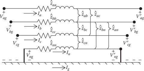
Figure 6.3
Three-phase line with neutral and ground currents.

In the development of the Kron reduction method, Equation 4.52 defined the “neutral transform matrix” $[t_{n}]$ . That equation is shown as Equation 6.44.

$[t_{n}] = - {[{\hat{z}}_{n n}]}^{- 1} \cdot [{\hat{z}}_{n j}]$ 6.44

The matrices $[{\hat{z}}_{n n}]$ and $[{\hat{z}}_{n j}]$ are the partitioned matrices in the primitive impedance matrix.

When the currents flowing in the lines have been determined, Equation 6.45 is used to compute the current flowing in the grounded neutral wire(s).

$[I_{n}] = [t_{n}] \cdot [I_{a b c}] .$ 6.45

In Equation 6.45, the matrix $[I_{n}]$ for an overhead line with one neutral wire will be a single element. However, in the case of an underground line consisting of concentric neutral cables or taped-shielded cables with or without a separate neutral wire, $[I_{n}]$ will be the currents flowing in each of the cable neutrals and the separate neutral wire if present. Once the neutral currents have been determined, Kirchhoff’s Current Law is used to compute the current flowing in the ground.

$I_{g} = - (I_{a} + I_{b} + I_{c} + I n_{1} + I n_{2} + \dots + I n_{k})$ 6.46

Example 6.2

The line of Example 6.1 will be used to supply an unbalanced load at node m. Assume that the voltages at the source end (node n) are balanced three-phase at 12.47 kV line-to-line. The balanced line-to-ground voltages are:

${[VLG]}_{n} = [\begin{matrix} 7199.56 \underset{_____}{/ 0} \\ 7199.56 \underset{_____}{/ - 120} \\ 7199.56 \underset{_____}{/ 120} \end{matrix}] V$

The unbalanced currents measured at the source end are given by:

${[\begin{matrix} I_{a} \\ I_{b} \\ I_{c} \end{matrix}]}_{n} = [\begin{matrix} 249.97 \underset{_____}{/ - 24.5} \\ 277.56 \underset{_____}{/ - 145.8} \\ 305.54 \underset{_____}{/ 95.2} \end{matrix}] A$

Determine the following:

The line-to-ground and line-to-line voltages at the load end (node m) using the modified line model
The voltage unbalance
The complex powers of the load
The currents flowing in the neutral wire and ground

Solution: The [A] and [B] matrices for the modified line model are:

$[A] = [U] = [\begin{matrix} 1 & 0 & 0 \\ 0 & 1 & 0 \\ 0 & 0 & 1 \end{matrix}]$

$[B] = [Z_{a b c}] = [\begin{matrix} 0.8666 + j 2.0417 & 0.2955 + j 0.9502 & 0.2907 + j 0.7290 \\ 0.2955 + j 0.9502 & 0.8837 + j 1.9852 & 0.2992 + j 0.8023 \\ 0.2907 + j 0.7290 & 0.2992 + j 0.8023 & 0.8741 + j 2.0172 \end{matrix}] Ω$

Because this is the approximate model, ${[I_{a b c}]}_{m}$ is equal to ${[I_{a b c}]}_{n.}$ Therefore:

${[\begin{matrix} I_{a} \\ I_{b} \\ I_{c} \end{matrix}]}_{m} = [\begin{matrix} 249.97 \underset{_____}{/ - 24.5} \\ 277.56 \underset{_____}{/ - 145.8} \\ 305.54 \underset{_____}{/ 95.2} \end{matrix}] A$

The line-to-ground voltages at the load end are:

${[VLG]}_{m} = [A] \cdot {[VLG]}_{n} - [B] \cdot {[I_{a b c}]}_{m} = [\begin{matrix} 6942.53 \underset{_____}{/ - 1.47} \\ 6918.35 \underset{_____}{/ - 121.55} \\ 6887.71 \underset{_____}{/ 117.31} \end{matrix}] V$

The line-to-line voltages at the load end are:

$[D v] = [\begin{matrix} 1 & - 1 & 0 \\ 0 & 1 & - 1 \\ - 1 & 0 & 1 \end{matrix}]$

${[V_{L L}]}_{m} = [D v] \cdot {[VLG]}_{m} = [\begin{matrix} 12, 008 \underset{_____}{/ 28.4} \\ 12, 025 \underset{_____}{/ - 92.2} \\ 11, 903 \underset{_____}{/ 148.1} \end{matrix}]$

For this condition, the average load voltage is:

$V_{average} = \frac{1}{3} \cdot \sum_{k = 1}^{3} {| VLG_{_{m}} |}_{k} = 6916.20$

The maximum deviation from the average is on phase c so that:

$\begin{array}{l} for: i = 1, 2, 3 \\ d V_{i} = | V_{average} - | VLG {_{_{m}}}_{_{i}} | | = [\begin{matrix} 26.33 \\ 2.15 \\ 28.49 \end{matrix}] \end{array}$

$V_{unbalance} = \frac{d V_{\max}}{V_{average}} = \frac{28.49}{6916.20} \cdot 100 = 0.4119 %$

The complex powers of the load are:

$[\begin{matrix} S_{a} \\ S_{b} \\ S_{c} \end{matrix}] = \frac{1}{1000} \cdot [\begin{matrix} V_{a g} \cdot I_{a}^{*} \\ V_{b g} . I_{b}^{*} \\ V_{c g} \cdot I_{c}^{*} \end{matrix}] = [\begin{matrix} 1597.2 + j 678.8 \\ 1750.8 + j 788.7 \\ 1949.7 + j 792.0 \end{matrix}] kW + j k v a r$

The “neutral transformation matrix” from Example 4.1 is:

$[t_{n}] = [\begin{matrix} - 0.4292 - j 0.1291 & - 0.4476 - j 0.1373 & - 0.4373 - j 0.1327 \end{matrix}]$

The neutral current is:

$[I_{n}] = [t_{n}] \cdot {[I_{a b c}]}_{m} = 26.2 \underset{_____}{/ - 29.5}$

The ground current is:

$I_{g} = - (I_{a} + I_{b} + I_{c} + I_{n}) = 32.5 \underset{_____}{/ - 77.6}$

6.3 The Approximate Line Segment Model

Many times, the only data available for a line segment will be the positive and zero sequence impedances. The approximate line model can be developed by applying the “reverse impedance transformation” from symmetrical component theory.

Using the known positive and zero sequence impedances, the “sequence impedance matrix” is given by:

$[Z_{seq}] = [\begin{matrix} Z_{0} & 0 & 0 \\ 0 & Z_{+} & 0 \\ 0 & 0 & Z_{+} \end{matrix}]$ 6.47

The “reverse impedance transformation” results in the following approximate phase impedance matrix.

$[Z_{a p p r o x}] = [A_{s}] \cdot [Z_{s e q}] \cdot {[A_{s}]}^{- 1}$ 6.48

$[Z_{a p p r o x}] = = \frac{1}{3} \cdot [\begin{matrix} (2 \cdot Z_{+} + Z_{0}) & (Z_{0} - Z_{+}) & (Z_{0} - Z_{+}) \\ (Z_{0} - Z_{+}) & (2 \cdot Z_{+} + Z_{0}) & (Z_{0} - Z_{+}) \\ (Z_{0} - Z_{+}) & (Z_{0} - Z_{+}) & (2 \cdot Z_{+} + Z_{0}) \end{matrix}]$ 6.49

Notice that the approximate impedance matrix is characterized by the three diagonal terms being equal and all mutual terms being equal. This is the same result that is achieved if the line is assumed to be transposed. Applying the approximate impedance matrix, the voltage at node n is computed to be:

${[\begin{matrix} V_{a g} \\ V_{b g} \\ V_{c g} \end{matrix}]}_{n} = {[\begin{matrix} V_{a g} \\ V_{b g} \\ V_{c g} \end{matrix}]}_{m} + \frac{1}{3} \cdot [\begin{matrix} (2 \cdot Z_{+} + Z_{0}) & (Z_{0} - Z_{+}) & (Z_{0} - Z_{+}) \\ (Z_{0} - Z_{+}) & (2 \cdot Z_{+} + Z_{0}) & (Z_{0} - Z_{+}) \\ (Z_{0} - Z_{+}) & (Z_{0} - Z_{+}) & (2 \cdot Z_{+} + Z_{0}) \end{matrix}] \cdot {[\begin{matrix} I_{a} \\ I_{b} \\ I_{c} \end{matrix}]}_{m}$ 6.50

In condensed form, Equation 6.50 becomes:

${[VLG]}_{n} = {[VLG]}_{m} + [Z_{approx}] \cdot {[I_{a b c}]}_{m}$ 6.51

Note that Equation 6.51 is of the form:

${[VLG]}_{n} = [a] {[VLG]}_{m} + [b] \cdot {[I_{a b c}]}_{m}$ 6.52

where:

[a] = unity matrix

[b] = [Z_approx]

Equation 6.50 can be expanded and an equivalent circuit for the approximate line segment model can be developed. Solving Equation 6.50 for the phase a voltage at node n results in:

$V_{a g}_{_{n}} = V_{a g}_{_{m}} + \frac{1}{3} {(2 Z_{+} + Z_{0}) I_{a} + (Z_{0} - Z_{+}) I_{b} + (Z_{0} + Z_{+}) I_{c}}$ 6.53

Modify Equation 6.53 by adding and subtracting the term $(Z_{0} - Z_{+}) I_{a}$ and then combining terms and simplifying:

$\begin{array}{l} V_{a g}_{_{n}} = V_{a g}_{_{m}} + \frac{1}{3} {\begin{cases} (2 Z_{+} + Z_{0}) I_{a} + (Z_{0} - Z_{+}) I_{b} + (Z_{0} - Z_{+}) I_{c} \\ + (Z_{0} - Z_{+}) I_{a} - (Z_{0} - Z_{+}) I_{a} \end{cases}} \\ V_{a g}_{_{n}} = V_{a g}_{_{m}} + \frac{1}{3} {(3 Z_{+}) I_{a} + (Z_{0} - Z_{+}) (I_{a} + I_{b} + I_{c})} \\ V_{a g}_{_{n}} = V_{a g}_{_{m}} + Z_{+} \cdot I_{a} + \frac{(Z_{0} - Z_{+})}{3} \cdot (I_{a} + I_{b} + I_{c}) \end{array}$ 6.54

The same process can be followed in expanding Equation 6.50 for phases b and c. The final results are:

$V_{b g}_{_{n}} = V_{b g}_{_{m}} + Z_{+} \cdot I_{b} + \frac{(Z_{0} - Z_{+})}{3} \cdot (I_{a} + I_{b} + I_{c})$ 6.55

$V_{c g}_{_{n}} = V_{c g}_{_{m}} + Z_{+} \cdot I_{c} + \frac{(Z_{0} - Z_{+})}{3} \cdot (I_{a} + I_{b} + I_{c})$ 6.56

Figure 6.4 illustrates the approximate line segment model.

images

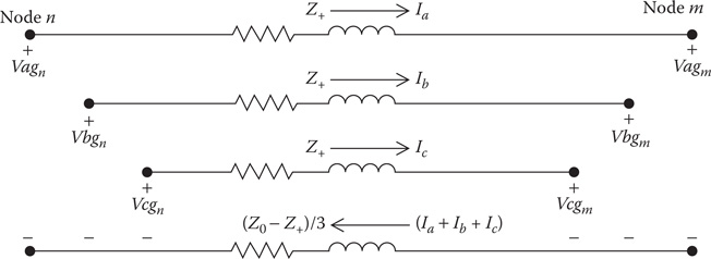
Figure 6.4
Approximate line segment model.

Figure 6.4 is a simple equivalent circuit for the line segment because no mutual coupling has to be modeled. It must be understood, however, that the equivalent circuit can only be used when transposition of the line segment has been assumed.

Example 6.3

The line segment of Example 4.1 is to be analyzed assuming that the line has been transposed. In Example 4.1, the positive and zero sequence impedances were computed to be:

$\begin{matrix} z_{+} = 0.3061 + j 0.6270 \\ z_{0} = 0.7735 + j 1.9373 \end{matrix} Ω /mile$

Assume that the load at node m is the same as in Example 6.1. That is:

$k V A = 6000, k V L L = 12.47, Power factor = 0.8 lagging$

Determine the voltages and currents at the source end (node n) for this loading condition.Solution: The sequence impedance matrix is:

$[z_{s e q}] = [\begin{matrix} 0.7735 + j 1.9373 & 0 & 0 \\ 0 & 0.3061 + j 0.6270 & 0 \\ 0 & 0 & 0.3061 + j 0.6270 \end{matrix}] Ω / m i l e$

Performing the reverse impedance transformation results in the approximate phase impedance matrix.

$[z_{a p p r o x}] = [A_{s}] \cdot [z_{s e q}] \cdot {[A_{s}]}^{- 1}$

$[z_{a p p r o x}] = [\begin{matrix} 0.4619 + j 1.0638 & 0.1558 + j 0.4368 & 0.1558 + j 0.4368 \\ 0.1558 + j 0.4368 & 0.4619 + j 1.0638 & 0.1558 + j 0.4368 \\ 0.1558 + j 0.4368 & 0.1558 + j 0.4368 & 0.4619 + j 1.0638 \end{matrix}] Ω /mile$

For the 10,000-ft line, the phase impedance matrix and the [b] matrix are:

$[b] = [Z_{approx}] = [z_{approx}] \cdot \frac{10, 000}{5280}$

$[b] = [\begin{matrix} 0.8748 + j 2.0147 & 0.2951 + j 0.8272 & 0.2951 + j 0.8272 \\ 0.2951 + j 0.8272 & 0.8748 + j 2.0147 & 0.2951 + j 0.8272 \\ 0.2951 + j 0.8272 & 0.2951 + j 0.8272 & 0.8748 + j 2.0147 \end{matrix}] Ω$

Note in the approximate phase impedance matrix that the three diagonal terms are equal and all of the mutual terms are equal. Again, this is an indication of the transposition assumption.

From Example 6.1, the voltages and currents at node m are:

${[VLG]}_{m} = [\begin{matrix} 7199.56 / \underset{___}{0} \\ 7199.56 \underset{_____}{/ - 120} \\ 7199.56 \underset{_____}{/ 120} \end{matrix}] V$

${[I_{a b c}]}_{m} = [\begin{matrix} 277.79 \underset{_____}{/ - 25.84} \\ 277.79 \underset{_____}{/ - 145.84} \\ 277.79 \underset{_____}{/ 94.16} \end{matrix}] A$

Using Equation 6.52:

${[VLG]}_{n} = [a] \cdot {[VLG]}_{m} + [b] \cdot {[I_{a b c}]}_{m} = [\begin{matrix} 7491.72 \underset{_____}{/ - 1.73} \\ 7491.72 \underset{_____}{/ - 118.27} \\ 7491.72 \underset{_____}{/ 121.73} \end{matrix}] V$

Note that the computed voltages are balanced. In Example 6.1, it was shown that when the line is modeled accurately, there is a voltage unbalance of 0.6275%. It should also be noted that the average value of the voltages at node n in Example 6.1 was 7491.69 V.

The V_ag at node n can also be computed using Equation 6.48.

$V_{a g}_{_{n}} = V_{a g}_{_{m}} + Z_{+} \cdot I_{a} + \frac{(Z_{0} - Z_{+})}{3} \cdot (I_{a} + I_{b} + I_{c})$

Because the currents are balanced, this equation reduces to:

$V_{a g}_{_{n}} = V_{a g}_{_{m}} + Z_{+} \cdot I_{a}$

$V_{a g}_{_{n}} = 7199.56 \underset{___}{/0} + (0.5797 + j 1.1875) \cdot 277.79 \underset{_____}{/ - 25.84} = 7491.72 \underset{_____}{/ 1.73} V$

It can be noted that when the loads are balanced and transposition has been assumed, the three-phase line can be analyzed as a simple single-phase equivalent as was done in the foregoing calculation.

Example 6.4

Use the balanced voltages and unbalanced currents at node n in Example 6.2 and the approximate line model to compute the voltages and currents at node m.Solution: From Example 6.2, the voltages and currents at node n are given as:

${[VLG]}_{n} = [\begin{matrix} 7199.56 \underset{_____}{/ 0} \\ 7199.56 \underset{_____}{/ - 120} \\ 7199.56 \underset{_____}{/ 120} \end{matrix}] V$

The [A] and [B] matrices for the approximate line model are:

where

$[A]$ =unity matrix

$[B] = [Z_{approx}]$

The voltages at node m are determined by:

${[VLG]}_{m} = [A] \cdot {[VLG]}_{n} - [B] \cdot {[I_{a b c}]}_{n} = [\begin{matrix} 6993.10 \underset{_____}{/ - 1.63} \\ 6881.15 \underset{_____}{/ - 121.61} \\ 6880.23 \underset{_____}{/ 117.50} \end{matrix}] V$

The voltage unbalance for this case is computed by:

$V_{average} = \frac{1}{3} \cdot \sum_{k = 1}^{3} {| VLG_{_{m}} |}_{k} = 6918.16$

$\begin{array}{l} for: i = 1, 2, 3 \\ d V_{i} = | V_{average} - | VLG {_{_{m}}}_{_{_{i}}} | | = [\begin{matrix} 74.94 \\ 37.01 \\ 37.93 \end{matrix}] \end{array}$

$V_{unbalance} = \frac{d V_{\max}}{V_{average}} = \frac{74.94}{6918.16} \cdot 100 = 1.0833 %$

Note that the approximate model has led to a higher voltage unbalance than the “exact” model.

6.4 The Modified “Ladder” Iterative Technique

The previous example problems have assumed a linear system. Unfortunately, that will not be the usual case for distribution feeders. When the source voltages are specified and the loads are specified as constant kW and kvar (constant PQ), the system becomes nonlinear and an iterative method will have to be used to compute the load voltages and currents. Chapter 10 develops in detail the modified “ladder” iterative technique. However, a simple form of that technique will be developed here in order to demonstrate how the nonlinear system can be evaluated.

The ladder technique is composed of two parts:

Forward sweep
Backward sweep

The forward sweep computes the downstream voltages from the source by applying Equation 6.57.

${[VLG_{_{a b c}}]}_{m} = [A] \cdot {[VLG_{_{a b c}}]}_{n} - [B] \cdot [I_{a b c}]$ 6.57

To start the process, the load currents

$[I_{a b c}]$ are assumed to be equal to zero and the load voltages are computed. In the first iteration, the load voltages will be the same as the source voltages and the load currents are computed.

The backward sweep computes the currents from the load back to the source using the most recently computed voltages from the forward sweep. Equation 6.58 is applied for this sweep.

$\begin{array}{l} {[I_{a b c}]}_{n} = [c] \cdot {[VLG_{_{a b c}}]}_{m} + [d] \cdot {[I_{a b c}]}_{m} \\ since: [c] = [0] \\ {[I_{a b c}]}_{n} = [d] \cdot {[I_{a b c}]}_{m} \end{array}$ 6.58

After the first forward and backward sweeps, the new load voltages are computed using the most recent currents. The forward and backward sweeps continue until the error between the new and previous load voltages are within a specified tolerance. Using the matrices computed in Example 6.1, a very simple Mathcad program that applies the ladder iterative technique is demonstrated in Example 6.5.

images

Figure 6.5
Mathcad program for Example 6.5.

Example 6.5

The line of Example 6.1 serves an unbalanced three-phase load of:

Phase a: 2500 kVA and PF = 0.9 lagging

Phase b: 2000 kVA and PF = 0.85 lagging

Phase c: 1500 kVA and PF = 0.95 lagging

The source voltages are balanced at 12.47 kV.

$\begin{array}{l} E_{L N} = \frac{12, 470}{\sqrt{3}} = 7199.6 \end{array}$

A simple Mathcad program (shown in Figure 6.5) is used to compute the load voltages and currents. The matrices [A] and [B] from Example 6.1 are used. After seven iterations, the load voltages and currents are computed to be:

$[VLG_{_{a b c}}] = [\begin{matrix} 66787.2 \underset{_____}{/ - 2.3} \\ 6972, 8 \underset{_____}{/ - 122.1} \\ 7055.5 \underset{_____}{/ 118.7} \end{matrix}] [I_{a b c}] = [\begin{matrix} 374.4 \underset{_____}{/ - 28.2} \\ 286.8 \underset{_____}{/ - 153.9} \\ 212.6 \underset{_____}{/ 100.5} \end{matrix}]$

Example 6.5 demonstrates the application of the ladder iterative technique. This technique will be used as models of other distribution feeder elements that are developed. A simple flowchart of the program and one that will be used in other chapters is shown in Figure 6.6.

images

Figure 6.6
Simple modified ladder flow chart.

6.5 The General Matrices for Parallel Lines

The equivalent Pi circuits for two parallel three-phase lines are shown in Figure 6.7.

images

Figure 6.7
Equivalent Pi parallel lines.

The 6 × 6 phase impedance and shunt admittance matrices for parallel three-phase lines were developed in Chapters 4 and 5. These matrices are used in the development of the general matrices used in modeling parallel three-phase lines.

The first step in computing the abcd matrices is to multiply the 6 × 6 phase impedance matrix from Chapter 4 and the 6 × 6 shunt admittance matrix from Chapter 5 by the distance that the lines are parallel.

$\begin{array}{l} [\begin{matrix} [v_{1}] \\ [v_{2}] \end{matrix}] = [\begin{matrix} [z_{11}] & [z_{12}] \\ [z_{21}] & [z_{22}] \end{matrix}] \cdot length \cdot [\begin{matrix} [I_{1}] \\ [I_{2}] \end{matrix}] = [\begin{matrix} [Z_{11}] & [Z_{12}] \\ [Z_{21}] & [Z_{22}] \end{matrix}] \cdot [\begin{matrix} [I_{1}] \\ [I_{2}] \end{matrix}] V \\ [v] = [Z] \cdot [I] \end{array}$ 6.59

$[\begin{matrix} [y_{11}] & [y_{12}] \\ [y_{21}] & [y_{22}] \end{matrix}] \cdot length = [\begin{matrix} [Y_{11}] & [Y_{12}] \\ [Y_{21}] & [Y_{22}] \end{matrix}] S$ 6.60

Referring to Figure 6.7, the line currents in the two circuits are given by:

$\begin{array}{l} [\begin{matrix} [I_{1}] \\ [I_{2}] \end{matrix}] = [\begin{matrix} [I_{R}_{_{1}}] \\ [I_{R}_{_{2}}] \end{matrix}] + \frac{1}{2} \cdot [\begin{matrix} [Y_{11}] & [Y_{12}] \\ [Y_{21}] & [Y_{22}] \end{matrix}] \cdot [\begin{matrix} [V_{R}_{_{1}}] \\ [V_{R}_{_{2}}] \end{matrix}] A \\ [I] = [I_{R}] + \frac{1}{2} \cdot [Y] \cdot [V_{R}] \end{array}$ 6.61

The sending end voltages are given by:

Substitute Equation 6.61 into Equation 6.62:

$\begin{array}{l} [\begin{matrix} [V_{S}_{_{1}}] \\ [V_{S}_{_{2}}] \end{matrix}] = [\begin{matrix} [V_{R}_{_{1}}] \\ [V_{R}_{_{2}}] \end{matrix}] + [\begin{matrix} [Z_{11}] & [Z_{12}] \\ [Z_{21}] & [Z_{22}] \end{matrix}] \cdot ([\begin{matrix} [I_{R}_{_{1}}] \\ [I_{R}_{_{2}}] \end{matrix}] + \frac{1}{2} \cdot [\begin{matrix} [Y_{11}] & [Y_{12}] \\ [Y_{21}] & [Y_{22}] \end{matrix}] \cdot [\begin{matrix} [V_{R}_{_{1}}] \\ [V_{R}_{_{2}}] \end{matrix}]) \\ [V_{S}] = [V_{R}] + [Z] \cdot ([I_{R}] + \frac{1}{2} \cdot [Y] \cdot [V_{R}]) \end{array}$ 6.63

Combine terms in Equation 6.63:

$\begin{array}{l} [\begin{matrix} [V_{S}_{_{1}}] \\ [V_{S}_{_{2}}] \end{matrix}] = ([\begin{matrix} [U] \\ [U] \end{matrix}] + \frac{1}{2} \cdot [\begin{matrix} [Z_{11}] & [Z_{12}] \\ [Z_{21}] & [Z_{22}] \end{matrix}] [\begin{matrix} [Y_{11}] & [Y_{12}] \\ [Y_{21}] & [Y_{22}] \end{matrix}]) \times [\begin{matrix} [V R_{1}] \\ [V R_{2}] \end{matrix}] + [\begin{matrix} [Z_{11}] & [Z_{12}] \\ [Z_{21}] & [Z_{22}] \end{matrix}] \cdot [\begin{matrix} [I R_{1}] \\ [I R_{2}] \end{matrix}] \\ [V_{S}] = ([U] + \frac{1}{2} \cdot [Z] \cdot [Y]) \cdot [V_{R}] + [Z] \cdot [I R] \end{array}$ 6.64

Equation 6.64 is of the form:

$[V_{S}] = [a] \cdot [V_{R}] + [b] \cdot [I_{R}]$ 6.65

where

$\begin{array}{l} [a] = [U] + \frac{1}{2} \cdot [Z] \cdot [Y] \\ [b] = [Z] \end{array}$ 6.66

The sending end currents are given by:

$\begin{array}{l} [\begin{matrix} [I_{S}_{_{1}}] \\ [I_{S}_{_{2}}] \end{matrix}] = [\begin{matrix} [I_{1}] \\ [I_{2}] \end{matrix}] + \frac{1}{2} \cdot [\begin{matrix} [Y_{11}] & [Y_{12}] \\ [Y_{21}] & [Y_{22}] \end{matrix}] \cdot [\begin{matrix} [V_{S}_{_{1}}] \\ [V_{S}_{_{2}}] \end{matrix}] \\ [I_{S}] = [I] + \frac{1}{2} \cdot [Y] \cdot [V_{S}] \end{array}$ 6.67

Substitute Equations 6.61 and 6.65 into Equation 6.67 using the shorthand form.

$[I_{S}] = [I_{R}] + \frac{1}{2} \cdot [Y] \cdot [V_{R}] + \frac{1}{2} \cdot [Y] \cdot ([a] \cdot [V_{R}] + [b] \cdot [I_{R}]) A$ 6.68

Combine terms in Equation 6.68.

$[I_{S}] = \frac{1}{2} \cdot ([Y] + [Y] \cdot [a]) \cdot [V_{R}] + ([U] + \frac{1}{2} \cdot [Y] \cdot [b]) \cdot [I_{R}]$ 6.69

Equation 6.69 is of the form:

$[I_{S}] = [c] \cdot [V_{R}] + [d] \cdot [I_{R}]$ 6.70

where

$\begin{array}{l} [c] = \frac{1}{2} \cdot ([Y] + [Y] \cdot [a]) = (\frac{1}{2} \cdot ([Y] + [Y] \cdot ([U] + \frac{1}{2} \cdot [Z] \cdot [Y]))) \\ [c] = [Y] + \frac{1}{4} \cdot [Y] \cdot [Z] \cdot [Y] \\ [d] = [U] + \frac{1}{2} \cdot [Y] \cdot [b] = [U] + \frac{1}{2} \cdot [Y] \cdot [Z] \end{array}$ 6.71

The derived matrices

$[a], [b], [c], [d]$ will be 6 × 6 matrices. These four matrices can all be partitioned between the third and fourth rows and columns. The final voltage equation in partitioned form is given by:

$[\begin{matrix} [V_{S}_{_{1}}] \\ [V_{S}_{_{2}}] \end{matrix}] = [\begin{matrix} [a_{11}] & [a_{12}] \\ [a_{21}] & [a_{22}] \end{matrix}] \cdot [\begin{matrix} [V_{R}_{_{1}}] \\ [V_{R}_{_{2}}] \end{matrix}] + [\begin{matrix} [b_{11}] & [b_{12}] \\ [b_{21}] & [b_{22}] \end{matrix}] \cdot [\begin{matrix} [I_{R}_{_{1}}] \\ [I_{R}_{_{2}}] \end{matrix}]$ 6.72

The final current equation in partitioned form is given by:

$[\begin{matrix} [I_{S}_{_{1}}] \\ [I_{S}_{_{2}}] \end{matrix}] = [\begin{matrix} [c_{11}] & [c_{12}] \\ [c_{21}] & [c_{22}] \end{matrix}] \cdot [\begin{matrix} [V_{R}_{_{1}}] \\ [V_{R}_{_{2}}] \end{matrix}] + [\begin{matrix} [d_{11}] & [d_{12}] \\ [d_{21}] & [d_{22}] \end{matrix}] \cdot [\begin{matrix} [I_{R}_{_{1}}] \\ [I_{R}_{_{2}}] \end{matrix}]$ 6.73

Equations 6.72 and 6.73 are used to compute the sending end voltages and currents of two parallel lines. The matrices [A] and [B] are used to compute the receiving end voltages when the sending end voltages and receiving end currents are known. Solving Equation 6.65 for [V_R]:

$\begin{array}{l} [V_{R}] = {[a]}^{- 1} \cdot ([V_{S}] - [b] \cdot [I_{R}]) \\ [V_{R}] = {[a]}^{- 1} \cdot [V_{S}] - {[a]}^{- 1} \cdot [b] \cdot [I_{R}] \\ [V_{R}] = [A] \cdot [V_{S}] - [B] \cdot [I_{R}] \end{array}$ 6.74

where

$\begin{array}{l} [A] = {[a]}^{- 1} \\ [B] = {[a]}^{- 1} \cdot [b] \end{array}$

In expanded form, Equation 6.74 becomes:

$[\begin{matrix} V_{R}_{_{1}} \\ V_{R}_{_{2}} \end{matrix}] = [\begin{matrix} [A_{11}] & [A_{12}] \\ [A_{21}] & [A_{22}] \end{matrix}] \cdot [\begin{matrix} V_{S}_{_{1}} \\ V_{S}_{_{2}} \end{matrix}] - [\begin{matrix} [B_{11}] & [B_{12}] \\ [B_{21}] & [B_{22}] \end{matrix}] \cdot [\begin{matrix} I_{R}_{_{1}} \\ I_{R}_{_{2}} \end{matrix}]$ 6.75

6.5.1 Physically Parallel Lines

Two distribution lines can be physically parallel in two different ways in a radial system. Figure 6.8 illustrates two lines connected to the same sending end node, but the receiving ends of the lines do not share a common node.

images

Figure 6.8
Physically parallel lines with a common sending end node.

The physically parallel lines of Figure 6.8 represent the common practice of two feeders leaving a substation on the same poles or right of ways and then branching in different directions downstream. Equations 6.72 and 6.73 are used to compute the sending end node voltages using the known line current flows and node voltages at the receiving end. For this special case, the sending end node voltages must be the same at the end of the two lines so that Equation 6.72 is modified to reflect that $[V_{S}_{_{1}}] = [V_{S}_{_{2}}]$ . A modified ladder iterative technique is used to force the two sending end voltages to be equal. In Chapter 10, the “ladder” iterative technique will be developed that will be used to adjust the receiving end voltages in such a manner that the sending end voltages will be the same for both lines.

Example 6.6

The parallel lines of Examples 4.2 and 5.2 are connected as shown in Figure 6.8 and are parallel to each other for 10 miles.

1. Determine the abcd and AB matrices for the parallel lines.

From Examples 4.2 and 5.2, the per-mile values of the phase impedance and shunt admittance matrices in partitioned form are shown. The first step is to multiply these matrices by the length of the line. Note that the units for the shunt admittance matrix in Example 5.2 are in μS/mile.

$\begin{array}{l} dist = 10 \\ Z = z \cdot dist \\ Y = y \cdot 10^{- 6} \cdot dist \end{array}$

The unit matrix [U] must be defined as 6 × 6, and then the abcd matrices are computed using the equations developed in this chapter. The final results in partitioned form are:

$[a_{11}] = [a_{22}] = [\begin{matrix} 0.9998 + j 0.0001 & 0 & 0 \\ 0 & 0.9998 + j 0.0001 & 0 \\ 0 & 0 & 0.9998 + j 0.0001 \end{matrix}]$

$[a_{12}] = [a_{21}] = [\begin{matrix} 0 & 0 & 0 \\ 0 & 0 & 0 \\ 0 & 0 & 0 \end{matrix}]$

$[b_{11}] = [\begin{matrix} 4.5015 + j 11.0285 & 1.4643 + j 5.3341 & 1.4522 + j 4.1255 \\ 1.4643 + j 5.3341 & 4.5478 + j 10.8726 & 1.4754 + j 4.5837 \\ 1.4522 + j 4.1255 & 1.4754 + j 4.5837 & 4.5231 + j 10.9556 \end{matrix}]$

$[b_{12}] = [\begin{matrix} 1.5191 + j 4.8484 & 1.4958 + j 3.9305 & 1.4775 + j 5.5601 \\ 1.5446 + j 5.3359 & 1.5205 + j 4.3234 & 1.5015 + j 4.9093 \\ 1.5311 + j 4.2867 & 1.5074 + j 5.4599 & 1.4888 + j 3.9548 \end{matrix}]$

$[b_{21}] = [\begin{matrix} 1.5191 + j 4.8484 & 1.5446 + j 5.3359 & 1.5311 + j 4.2867 \\ 1.4958 + j 3.9305 & 1.5205 + j 4.3234 & 1.5074 + j 5.4599 \\ 1.4775 + j 5.5601 & 1.5015 + j 4.9093 & 1.4888 + j 3.9548 \end{matrix}]$

$[b_{22}] = [\begin{matrix} 5.7063 + j 10.9130 & 1.5801 + j 4.2365 & 1.5595 + j 5.0167 \\ 1.5801 + j 4.2365 & 5.6547 + j 11.0819 & 1.5348 + j 3.8493 \\ 1.5595 + j 5.0167 & 1.5348 + j 3.8493 & 5.6155 + j 11.2117 \end{matrix}]$

$\begin{array}{l} [c_{11}] = [c_{12}] = [\begin{matrix} j 0.0001 & 0 & 0 \\ 0 & j 0.0001 & 0 \\ 0 & 0 & j 0.0001 \end{matrix}] \\ [c_{21}] = [c_{22}] = [\begin{matrix} 0 & 0 & 0 \\ 0 & 0 & 0 \\ 0 & 0 & 0 \end{matrix}] \end{array}$

$[d_{11}] = [a_{11}] [d_{12}] = [a_{12}] [d_{21}] = [a_{21}] [d_{22}] = [a_{22}]$

$[A_{11}] = [A_{22}] = {[a_{11}]}^{- 1} = [\begin{matrix} 1.0002 - j 0.0001 & 0 & 0 \\ 0 & 1.0002 - j 0.0001 & 0 \\ 0 & 0 & 1.0002 - j 0.0001 \end{matrix}]$

$[A_{12}] = [A_{21}] = [\begin{matrix} 0 & 0 & 0 \\ 0 & 0 & 0 \\ 0 & 0 & 0 \end{matrix}]$

$[B_{11}] = {[a_{11}]}^{- 1} \cdot [b_{11}] = [\begin{matrix} 4.5039 + j 11.031 & 1.4653 + j 5.3357 & 1.4533 + j 4.1268 \\ 1.4653 + j 5.3357 & 4.5502 + j 10.8751 & 1.4764 + j 4.5852 \\ 1.4533 + j 4.1268 & 1.4764 + j 4.5852 & 4.5255 + j 10.9580 \end{matrix}]$

$[B_{12}] = {[a_{12}]}^{- 1} \cdot [b_{12}] = [\begin{matrix} 1.5202 + j 4.8499 & 1.4969 + j 3.9318 & 1.4786 + j 5.5618 \\ 1.4969 + j 3.9318 & 1.5216 + j 4.3248 & 1.5026 + j 4.9108 \\ 1.4786 + j 5.5618 & 1.5026 + j 4.9108 & 1.4899 + j 3.9560 \end{matrix}]$

$[B_{21}] = {[a_{21}]}^{- 1} \cdot [b .21] = [\begin{matrix} 1.5202 + j 4.8499 & 1.5457 + j 5.3375 & 1.5322 + j 4.2881 \\ 1.5457 + j 5.3375 & 1.5216 + j 4.3248 & 1.5058 + j 5.4615 \\ 1.5322 + j 4.2881 & 1.5058 + j 5.4615 & 1.4899 + j 3.9560 \end{matrix}]$

$[B_{22}] = {[a_{22}]}^{- 1} \cdot [b_{22}] = [\begin{matrix} 5.7092 + j 10.9152 & 1.5812 + j 4.2378 & 1.5606 + j 5.0183 \\ 1.5812 + j 4.2378 & 5.6577 + j 11.0842 & 1.5360 + j 3.8506 \\ 1.5606 + j 5.0183 & 1.5360 + j 3.8506 & 5.6184 + j 11.2140 \end{matrix}]$

The loads at the ends of the two lines are treated as constant current loads with values of: Line 1:

$[I_{R}_{_{1}}] = [\begin{matrix} 102.6 \underset{_____}{/ - 20.4} \\ 82.1 \underset{_____}{/ - 145.2} \\ 127.8 \underset{_____}{/ 85.2} \end{matrix}]$

Line 2:

$[I_{R}_{_{2}}] = [\begin{matrix} 94.4 \underset{_____}{/} \underset{_____}{- 27.4} \\ 127.4 \underset{_____}{/ - 152.5} \\ 100.2 \underset{_____}{/ 99.8} \end{matrix}]$

The voltages at the sending end of the lines are:

$[V_{S}] = [\begin{matrix} 14, 400 \underset{_____}{/ 0} \\ 14, 400 \underset{_____}{/ - 120} \\ 14, 400 \underset{_____}{/ 120} \end{matrix}]$

2. Determine the receiving end voltages for the two lines.

Because the common sending end voltages are known and the receiving end line currents are known, Equation 6.75 is used to compute the receiving end voltages: Line 1:

$\begin{array}{l} [V_{R}_{_{1}}] = ([A_{11}] + [A_{12}]) \cdot [V_{S}] - [B_{11}] \cdot [I_{R}_{_{1}}] - [B_{12}] \cdot [I_{R}_{_{2}}] \\ [V_{R}_{_{1}}] = [\begin{matrix} 14, 119 \underset{_____}{/ - 2.3} \\ 14, 022 \underset{_____}{/ - 120.4} \\ 13, 686 \underset{_____}{/ 117.4} \end{matrix}] \end{array}$

Line 2:

$\begin{array}{l} [V_{R}_{_{2}}] = ([A_{21}] + [A_{22}]) \cdot [V_{1}] - [B_{21}] \cdot [I_{R}_{_{1}}] - [B_{22}] \cdot [I_{R}_{_{2}}] \\ [V_{R}_{_{2}}] = [\begin{matrix} 13, 971 \underset{_____}{/ - 1.6} \\ 13, 352 \underset{_____}{/ - 120.8} \\ 13, 566 \underset{_____}{/ 118.1} \end{matrix}] \end{array}$

The second way in which two lines can be physically parallel in a radial feeder is to have neither the sending nor the receiving ends common to both lines. This is shown in Figure 6.9.

images

Figure 6.9
Physically parallel lines without common nodes.

Equations 6.72 and 6.73 are again used for the analysis of this special case. Because neither the sending end nor the receiving end nodes are common, no adjustments need to be made to Equation 6.72. Typically, these lines will be part of a large distribution feeder in which case an iterative process will be used to arrive at the final values of the sending and receiving end voltages and currents.

Example 6.7

The parallel lines of Examples 4.2 and 5.2 are connected as shown in Figure 6.9. The lines are parallel to each other for 10 miles.

The complex power flowing out of each line is:

Line 1:

$\begin{array}{l} S_{1}_{_{a}} = 1450 kVA, P F_{a} = 0.95 \\ S_{1}_{_{b}} = 1150 kVA, P F_{b} = 0.90 \\ S_{1}_{_{c}} = 1750 kVA, P F_{c} = 0.85 \end{array}$

Line 2:

$\begin{array}{l} S_{2}_{_{a}} = 1320 kVA, P F_{a} = 0.90 \\ S_{2}_{_{b}} = 1700 kVA, P F_{b} = 0.85 \\ S_{2}_{_{c}} = 1360 kVA, P F_{c} = 0.95 \end{array}$

The line-to-neutral voltages at the receiving end nodes are:

Line 1:

$\begin{array}{l} V_{R} {_{_{1}}}_{_{_{a n}}} = 13, 430 \underset{_____}{/ - 33.1} \\ V_{R} {_{_{1}}}_{_{_{b n}}} = 13, 956 \underset{_____}{/ - 151.3} \\ V_{R} {_{_{1}}}_{_{_{c n}}} = 14, 071 \underset{_____}{/ 86.0} \end{array}$

Line 2:

$\begin{array}{l} V_{R} {_{_{2}}}_{_{_{a n}}} = 14, 501 \underset{_____}{/ - 29.1} \\ V_{R} {_{_{2}}}_{_{_{b n}}} = 13, 932 \underset{_____}{/ - 154.8} \\ V_{R} {_{_{2}}}_{_{_{c n}}} = 12, 988 \underset{_____}{/ 90.3} \end{array}$

Determine the sending end voltages of the two lines.

The currents leaving the two lines are:

Line 1:

$\begin{array}{l} For i = a, b, c \\ I_{R} {_{_{1}}}_{_{_{i}}} = {(\frac{S_{1}_{_{i}} \cdot 1000}{V_{1}_{_{i}}})}^{*} = [\begin{matrix} 108.0 \underset{_____}{/ - 51.3} \\ 82.4 \underset{_____}{/ - 177.1} \\ 124.4 \underset{_____}{/ 54.2} \end{matrix}] \end{array}$

Line 2:

$\begin{array}{l} For i = a, b, c \\ I_{R} {_{_{2}}}_{_{_{i}}} = {(\frac{S_{2}_{_{i}} \cdot 1000}{V_{2}_{_{i}}})}^{*} = [\begin{matrix} 91.0 \underset{_____}{/ - 54.9} \\ 122.0 \underset{_____}{/ 173.5} \\ 104.7 \underset{_____}{/ 72.1} \end{matrix}] \end{array}$

The sending end voltages of the two lines are computed using Equation 6.72.

Line 1:

$[V_{S}_{_{1}}] = [\begin{matrix} 13, 673 \underset{_____}{/ - 30.5} \\ 14, 361 \underset{_____}{/ - 151.0} \\ 14, 809 \underset{_____}{/ 88.7} \end{matrix}]$

Line 2:

$[V_{S}_{_{2}}] = [\begin{matrix} 14, 845 \underset{_____}{/ - 27.5} \\ 14, 973 \underset{_____}{/ - 154.3} \\ 13, 898 \underset{_____}{/ 92.5} \end{matrix}]$

The sending end currents are:

$[I_{S}_{_{1}}] = [\begin{matrix} 107.7 \underset{_____}{/ - 50.8} \\ 82.0 \underset{_____}{/ - 176.2} \\ 124.0 \underset{_____}{/ 54.7} \end{matrix}]$

$[I_{S}_{_{2}}] = [\begin{matrix} 90.5 \underset{_____}{/ - 54.3} \\ 121.4 \underset{_____}{/ 173.8} \\ 104.2 \underset{_____}{/ 72.6} \end{matrix}]$

Note in this example the very slight difference between the sending and receiving end currents. The very small difference is because of the shunt admittance. It is seen that very little error will be made if the shunt admittance of the two lines is ignored. This will be the usual case. Exceptions will be for very long distribution lines (50 miles or more) and for underground concentric neutral lines that are in parallel for 10 miles or more

A third option for physically parallel lines in a radial feeder might be considered with the receiving end nodes common to both lines and the sending end nodes not common. However, this would violate the “radial” nature of the feeder, since the common receiving end nodes would constitute the creation of a loop.

6.5.2 Electrically Parallel Lines

Figure 6.10 shows two distribution lines that are electrically parallel.

The analysis of the electrically parallel lines requires an extra step from that of the physically parallel lines, since the individual line currents are not known. In this case, only the total current leaving the parallel lines is known.

images

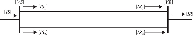
Figure 6.10
Electrically parallel lines.

In the typical analysis, the receiving end voltages will either have been assumed or computed, and the total phase currents $[I_{R}]$ will be known. With $[V_{S}]$ and $[V_{R}]$ common to both lines, the first step must be to determine how much of the total current $[I_{R}]$ flows on each line. Because the lines are electrically parallel, Equation 6.72 can be modified to reflect this condition:

$[\begin{matrix} [V_{S}] \\ [V_{S}] \end{matrix}] = [\begin{matrix} [a_{11}] & [a_{12}] \\ [a_{21}] & [a_{22}] \end{matrix}] \cdot [\begin{matrix} [V_{R}] \\ [V_{R}] \end{matrix}] + [\begin{matrix} [b_{11}] & [b_{12}] \\ [b_{21}] & [b_{22}] \end{matrix}] \cdot [\begin{matrix} [I_{R}_{_{1}}] \\ [I_{R}_{_{2}}] \end{matrix}]$ 6.76

The current in line 2 is a function of the total current, and the current in line 1 is given by:

$[I_{R}_{_{2}}] = [I_{R}] - [I_{R}_{_{1}}]$ 6.77

Substitute Equation 6.77 into Equation 6.76:

Because the sending end voltages are equal, Equation 6.78 is modified to reflect this:

$([a_{11}] + [a_{12}]) \cdot [V_{R}] + ([b_{11}] - [b_{12}]) \cdot [I_{R}_{_{1}}] + [b_{12}] \cdot [I_{R}] = ([a_{21}] + [a_{22}]) \cdot [V_{R}] + ([b_{21}] - [b_{22}]) \cdot [I_{R}_{_{1}}] + [b_{22}] \cdot [I_{R}]$ 6.79

Collect terms in Equation 6.79:

$([a_{11}] + [a_{12}] - [a_{21}] - [a_{22}]) \cdot [V_{R}] + ([b_{12}] - [b_{22}]) \cdot [I_{R}] = ([b_{21}] - [b_{22}] - [b_{11}] + [b_{12}]) \cdot [I_{R}_{_{1}}]$ 6.80

Equation 6.80 is in the form of:

$[A_{a}] \cdot [V_{R}] + [B_{b}] \cdot [I_{R}] = [C_{b}] \cdot [I_{R}_{_{1}}]$ 6.81

where

$\begin{array}{l} [A_{a}] = [a_{11}] + [a_{12}] - [a_{21}] - [a_{22}] \\ [B_{b}] = [b_{12}] - [b_{22}] \\ [C_{c}] = [b_{21}] - [b_{22}] - [b_{11}] + [b_{12}] \end{array}$ 6.82

Equation 6.81 can be solved for the receiving end current in line 1:

$[I_{R}_{_{1}}] = {[C_{c}]}^{- 1} \cdot ([A_{a}] \cdot [V_{R}] + [B_{b}] \cdot [I_{R}])$ 6.83

Equation 6.77 can be used to compute the receiving end current in line 2.

With the two receiving end line currents known, Equations 6.72 and 6.73 are used to compute the sending end voltages. As with the physically parallel lines, an iterative process (Chapter 10) will have to be used to ensure that the sending end voltages for each line are equal.

Example 6.8

The two lines in Example 6.5 are electrically parallel as shown in Figure 6.10. The receiving end voltages are given by:

$[V_{R}] = [\begin{matrix} 13, 280 \underset{_____}{/ - 33.1} \\ 14, 040 \underset{_____}{/ 151.7} \\ 14, 147 \underset{_____}{/ 86.5} \end{matrix}]$

The complex power-out of the parallel lines is the sum of the complex power of the two lines in Example 6.6:

$\begin{array}{l} S_{a} = 2, 763.8 kVA at 0.928 P F \\ S_{b} = 2, 846.3 kVA at 0.872 P F \\ S_{c} = 3, 088.5 kVA at 0.90 P F \end{array}$

The first step in the solution is to determine the total current leaving the two lines:

$I_{R}_{_{i}} = {(\frac{S_{i} \cdot 1000}{V_{R}_{_{i}}})}^{*} = [\begin{matrix} 208.1 \underset{_____}{/ - 54.9} \\ 202.7 \underset{_____}{/ 179.0} \\ 218.8 \underset{_____}{/ 50.2} \end{matrix}]$

Equation 6.83 is used to compute the current in line 1. Before that is done, the matrices of Equation 6.82 must be computed.

$\begin{array}{l} [A_{a}] = [a_{11}] + [a_{12}] - [a_{21}] - [a_{22}] = [\begin{matrix} 0 & 0 & 0 \\ 0 & 0 & 0 \\ 0 & 0 & 0 \end{matrix}] \\ [B_{b}] = [b_{12}] - [b_{22}] = [\begin{matrix} - 4.1872 - j 6.0646 & - 0.0843 - j 0.3060 & - 0.0820 + j 0.5434 \\ - 0.0354 + j 1.0995 & - 4.1342 - j 6.7585 & - 0.0333 + j 1.0599 \\ - 0.0284 - j 0.7300 & - 0.0274 + j 1.6105 & - 4.1267 - j 7.2569 \end{matrix}] \\ [C_{c}] = [b_{21}] - [b_{22}] - [b_{11}] + [b_{12}] = [\begin{matrix} - 7.1697 - j 12.2446 & - 0.0039 - j 0.3041 & - 0.0032 + j 0.7046 \\ - 0.0039 - j 0.3041 & - 7.1616 - j 13.3077 & - 0.0013 + j 1.9361 \\ - 0.0032 + j 0.7046 & - 0.0013 + j 1.9361 & - 7.1610 - j 14.2577 \end{matrix}] \end{array}$

The current in line 1 is now computed by:

$[I_{R}_{_{1}}] = {[C_{c}]}^{- 1} \cdot ([A_{a}] \cdot [V_{R}] + [B_{b}] \cdot [I_{R}]) = [\begin{matrix} 110.4 \underset{_____}{/ - 59.7} \\ 119.3 \underset{_____}{/ 172.6} \\ 121.7 \underset{_____}{/ 50.2} \end{matrix}]$

The current in line 2 is:

$[I_{R}_{_{2}}] = [I_{R}] - [I_{R}_{_{1}}] = [\begin{matrix} 98.5 \underset{_____}{/ - 49.6} \\ 85.2 \underset{_____}{/ - 172.2} \\ 101.1 \underset{_____}{/ 73.3} \end{matrix}]$

The sending end voltages are:

$\begin{array}{l} [V_{S}_{_{1}}] = ([a_{11}] + [a_{12}]) \cdot [V_{R}] + [b_{11}] \cdot [I_{R}_{_{1}}] + [b_{12}] \cdot [I_{R}_{_{2}}] = [\begin{matrix} 13, 738 \underset{_____}{/ - 30.9} \\ 14, 630 \underset{_____}{/ - 151.0} \\ 14, 912 \underset{_____}{/ 88.3} \end{matrix}] \\ [V_{S}_{_{2}}] = ([a_{21}] + [a_{22}]) \cdot [V_{R}] + [b_{21}] \cdot [I_{R}_{_{1}}] + [b_{22}] \cdot [I_{R}_{_{2}}] = [\begin{matrix} 13, 738 \underset{_____}{/ - 30.9} \\ 14, 630 \underset{_____}{/ - 151.0} \\ 14, 912 \underset{_____}{/ 88.3} \end{matrix}] \end{array}$

It is satisfying that the two equations give us the same results for the sending end voltages.

The sending end currents are:

$\begin{array}{l} [I_{S}_{_{1}}] = ([c_{11}] + [c_{12}]) \cdot [V_{R}] + [d_{11}] \cdot [I_{R}_{_{1}}] + [d_{12}] \cdot [I_{R}_{_{2}}] = [\begin{matrix} 110.0 \underset{_____}{/ - 59.2} \\ 118.7 \underset{_____}{/ 173.1} \\ 121.2 \underset{_____}{/ 50.6} \end{matrix}] \\ [I_{S}_{_{2}}] = ([c_{21}] + [c_{22}]) \cdot [V_{R}] + [d_{21}] \cdot [I_{R}_{_{1}}] + [d_{22}] \cdot [I_{R}_{_{2}}] = [\begin{matrix} 98.2 \underset{_____}{/ - 49.0} \\ 84.7 \underset{_____}{/ - 171.7} \\ 100.7 \underset{_____}{/ 73.9} \end{matrix}] \end{array}$

When the shunt admittance of the parallel lines is ignored, a parallel equivalent 3 ×3 phase impedance matrix can be determined. Because very little error is made ignoring the shunt admittance on most distribution lines, the equivalent parallel phase impedance matrix can be very useful in distribution power flow programs that are not designed to model electrically parallel lines.

Because the lines are electrically parallel, the voltage drops in the two lines must be equal. The voltage drop in the two parallel lines is given by:

$[\begin{matrix} [V_{a b c}] \\ [V_{a b c}] \end{matrix}] = [\begin{matrix} [Z_{11}] & [Z_{12}] \\ [Z_{21}] & [Z_{22}] \end{matrix}] \cdot [\begin{matrix} I_{R}_{_{1}} \\ I_{R}_{_{2}} \end{matrix}]$ 6.84

Substitute Equation 6.77 into Equation 6.84:

$[\begin{matrix} [V_{a b c}] \\ [V_{a b c}] \end{matrix}] = [\begin{matrix} [Z_{11}] & [Z_{12}] \\ [Z_{21}] & [Z_{22}] \end{matrix}] \cdot [\begin{matrix} [I_{R}_{_{1}}] \\ [I_{R}] - [I_{R}_{_{1}}] \end{matrix}]$ 6.85

Expand Equation 6.85 to solve for the voltage drops:

$\begin{array}{l} [V_{a b c}] = [Z_{11}] \cdot [I_{R}_{_{1}}] + [Z_{12}] \cdot ([I_{R}] - [I_{R}_{_{1}}]) = [Z_{21}] \cdot [I_{R}_{_{1}}] + [Z_{22}] \cdot ([I_{R}] - [I_{R}_{_{1}}]) \\ [V_{a b c}] = ([Z_{11}] - [Z_{12}]) \cdot [I_{R}_{_{1}}] + [Z_{12}] \cdot [I_{R}] = ([Z_{21}] - [Z_{22}]) \cdot [I_{R}_{_{1}}] + [Z_{22}] \cdot [I_{R}] \end{array}$ 6.86

Collect terms in Equation 6.86:

$([Z_{11}] - [Z_{12}] - [Z_{21}] + [Z_{22}]) \cdot [I_{R}_{_{1}}] = ([Z_{22}] - [Z_{12}]) \cdot [I_{R}]$ 6.87

Let:

$[Z_{X}] = ([Z_{11}] - [Z_{12}] - [Z_{21}] + [Z_{22}])$ 6.88

Substitute Equation 6.88 into Equation 6.87, and solve for the current in line 1:

$[I_{R}_{_{1}}] = {[Z_{X}]}^{- 1} \cdot ([Z_{22}] - [Z_{12}]) \cdot [I_{R}]$ 6.89

Substitute Equation 6.89 into the top line of Equation 6.85.

$[V_{a b c}] = (([Z_{11} - Z_{12}]) \cdot {[Z_{X}]}^{- 1} \cdot ([Z_{22}] - [Z_{12}]) + [Z_{12}]) \cdot [I_{R}]$ 6.90

$\begin{array}{l} [V_{a b c}] = [Z_{eq}] \cdot [I_{R}] \end{array}$ 6.91

where

$[Z_{eq}] = (([Z_{11} - Z_{12}]) \cdot {[Z_{X}]}^{- 1} \cdot ([Z_{22}] - [Z_{12}]) + [Z_{12}])$

The equivalent impedance of Equation 6.91 is the 3 ×3 equivalent for the two lines that are electrically parallel. This is the phase impedance matrix that can be used in conventional distribution power flow programs that cannot model electrically parallel lines.

Example 6.9

The same two lines are electrically parallel, but the shunt admittance is neglected. Compute the equivalent 3 ×3 impedance matrix using the impedance-partitioned matrices of Example 6.6.

$[Z_{X}] = [Z_{11}] - [Z_{12}] - [Z_{21}] + [Z_{22}] = [\begin{matrix} 7.1697 + j 12.2446 & 0.0039 + j 0.3041 & 0.0032 - j 0.7046 \\ 0.0039 + j 0.3041 & 7.1616 + j 13.3077 & 0.0013 - j 1.9361 \\ 0.0032 - j 0.7046 & 0.0013 - j 1.9361 & 7.1610 + j 14.2577 \end{matrix}]$

$[Z_{eq}] = ([Z_{11}] - [Z_{12}]) \cdot {[Z_{X}]}^{- 1} \cdot ([Z_{22}] - [Z_{12}]) + [Z_{12}] = [\begin{matrix} 3.3677 + j 7.796 & 1.5330 + j 4.7717 & 1.4867 + j 4.7304 \\ 1.5330 + j 4.7717 & 3.3095 + j 7.6459 & 1.5204 + j 4.7216 \\ 1.4867 + j 4.7304 & 1.5204_j 4.7216 & 3.2662 + j 7.5316 \end{matrix}]$

The sending end voltages are:

$[V_{S}] = [V_{R}] + [Z_{eq}] \cdot [I_{R}] = [\begin{matrix} 13, 740 \underset{_____}{/ - 31.0} \\ 14, 634 \underset{_____}{/ - 151.0} \\ 14, 916 \underset{_____}{/ 88.3} \end{matrix}]$

6.6 Summary

This chapter has developed the “exact,” “modified,” and “approximate” line segment models. The exact model uses no approximations. That is, the phase impedance matrix, assuming no transposition, and the shunt admittance matrix are used. The modified model ignores the shunt admittance. The approximate line model ignores the shunt admittance and assumes that the positive and zero sequence impedances of the line are the known parameters. This is paramount to assuming the line is transposed. For the three line models, generalized matrix equations have been developed. The equations utilize the generalized matrices [a],[b],[c],[d],[A] and [B]. The example problems demonstrate that because the shunt admittance is very small, the generalized matrices can be computed by neglecting the shunt admittance with very little, if any, error. In most cases, the shunt admittance can be neglected; however, there are situations where the shunt admittances should not be neglected. This is particularly true for long, rural, lightly loaded lines and for many underground lines.

A method for computing the current flowing in the neutral and ground was developed. The only assumption used that can make a difference on the computing currents is that the resistivity of earth was assumed to be 100 Ω-m.

A simple version of the ladder iterative technique was introduced and applied in Example 6.5. The ladder method will be used in future chapters and is fully developed in Chapter 10.

The generalized matrices for two lines in parallel have been derived. The analysis of physically parallel and electrically parallel lines was developed with examples to demonstrate the analysis process.

Problems

6.1 A 2-mile long three-phase line uses the configuration of Problem 4.1. The phase impedance matrix and shunt admittance matrix for the configuration are:

$[z_{a b c}] = [\begin{matrix} 0.3375 + j 1.0478 & 0.1535 + j 0.3849 & 0.1559 + j 0.5017 \\ 0.1535 + j 0.3849 & 0.3414 + j 1.0348 & 0.1580 + j 0.4236 \\ 0.1559 + j 0.5017 & 0.1580 + j 0.4236 & 0.3465 + j 1.0179 \end{matrix}] Ω / mile$

$[y_{a b c}] = [\begin{matrix} j 5.9540 & - j 0.7471 & - j 2.0030 \\ - j 0.7471 & j 5.6322 & - j 1.2641 \\ - j 2.0030 & - j 1.2641 & j 6.3962 \end{matrix}] μ S/mile$

The line is serving a balanced three-phase load of 10,000 kVA, with balanced voltages of 13.2 kV line-to-line, and a power factor of 0.85 lagging.

a. Determine the generalized matrices.
b. For the given load, compute the line-to-line and line-to-neutral voltages at the source end of the line.
c. Compute the voltage unbalance at the source end.
d. Compute the source end complex power per phase.
e. Compute the power loss by phase over the line. (Hint: Power loss is defined as power-in minus power-out)

6.2 Use the line of Problem 6.1. For this problem, the source voltages are specified as:

$[V_{S}_{_{LN}}] = [\begin{matrix} 7620 \underset{_____}{/ 0} \\ 7620 \underset{_____}{/ - 120} \\ 7620 \underset{_____}{/ 120} \end{matrix}]$

The three-phase load is unbalanced connected in wye and given by:

$[k V A] = [\begin{matrix} 2500 \\ 3500 \\ 1500 \end{matrix}] [P F] = [\begin{matrix} 0.90 \\ 0.85 \\ 0.95 \end{matrix}]$

Use the ladder iterative technique and determine:

a. The load line-to-neutral voltages
b. Power at the source
c. The voltage unbalance at the load

6.3 Use WindMil for Problem 6.2.

6.4 The positive and zero sequence impedances for the line in Problem 6.1 are:

$z_{+} = 0.186 + j 0.5968 Ω/mile, z_{0} = 0.6534 + j 1.907 Ω/mile$

Repeat Problem 6.1 using the “approximate” line model.

6.5 The line of Problem 6.1 serves an unbalanced grounded wye connected constant impedance load of:

$Z_{a g} = 15 / \underset{_____}{30} Ω, Z_{b g} = 17 / \underset{_____}{36.87} Ω, Z_{c g} = 20 / \underset{_____}{25.84} Ω$

The line is connected to a balanced three-phase 13.2 kV source.

Determine the load currents.
Determine the load line-to-ground voltages.
Determine the complex power of the load by phase.
Determine the source complex power by phase.
Determine the power loss by phase and the total three-phase power loss.
Determine the current flowing in the neutral and ground.

6.6 Repeat Problem 6.3; only the load on phase b is changed to 50/36.87 Ω.

6.7 The two-phase line of Problem 4.2 has the following phase impedance matrix:

$[z_{a b c}] = [\begin{matrix} 0.4576 + j 1.0780 & 0 & 0.1535 + j 0.3849 \\ 0 & 0 & 0 \\ 0.1535 + j 0.3849 & 0 & 0.4615 + j 1.0651 \end{matrix}] Ω /mile$

The line is 2 miles long and serves a two-phase load such that:

S _ag = 2000 kVA at 0.9 lagging power factor and voltage of 7620/0 V

S _cg = 1500 kVA at 0.95 lagging power factor and voltage of 7620/120 V

Neglect the shunt admittance and determine the following:

The source line-to-ground voltages using the generalized matrices. (Hint: Even though phase b is physically not present, assume that it is with a value of 7620/−120 V and is serving a 0 kVA load.)
The complex power by phase at the source.
The power loss by phase on the line.
The current flowing in the neutral and ground.

6.8 The single-phase line of Problem 4.3 has the following phase impedance matrix:

$[z_{a b c}] = [\begin{matrix} 0 & 0 & 0 \\ 0 & 1.3292 + j 1.3475 & 0 \\ 0 & 0 & 0 \end{matrix}] Ω /mile$

The line is 1 mile long and serves a single-phase load of 2000 kVA, 0.95 lagging power factor at a voltage of 7500/−120 V. Determine the source voltage and power loss on the line. (Hint: As in the previous problem, even though phases a and c are not physically present, assume they are and along with phase b make up a balanced three-phase set of voltages.)

6.9 The three-phase concentric neutral cable configuration of Problem 4.10 is two miles long and serves a balanced three-phase load of 10,000 kVA, 13.2 kV, 0.85 lagging power factor. The phase impedance and shunt admittance matrices for the cable line are:

$[z_{a b c}] = [\begin{matrix} 0.7891 + j 0.4041 & 0.3192 + j 0.0328 & 0.3192 + j 0.0328 \\ 0.3192 + j 0.0328 & 0.7982 + j 0.4463 & 0.2849 - j 0.0143 \\ 0.3192 + j 0.0328 & 0.2849 - j 0.0143 & 0.8040 + j 0.4381 \end{matrix}] Ω /mile$

$[y_{a b c}] = [\begin{matrix} j 96.61 & 0 & 0 \\ 0 & j 96.61 & 0 \\ 0 & 0 & j 96.61 \end{matrix}] μ S/mile$

a. Determine the generalized matrices.
b. For the given load, compute the line-to-line and line-to-neutral voltages at the source end of the line.
c. Compute the voltage unbalance at the source end.
d. Compute the source end complex power per phase.
e. Compute the power loss by phase over the line. (Hint: Power loss is defined as power-in minus power-out.)

6.10 The line of Problem 6.9 serves an unbalanced grounded wye connected constant impedance load of:

Z_ag = 15/30 Ω, Z_bg = 50/36.87 Ω, Z_cg = 20/25.84 Ω

The line is connected to a balanced three-phase 13.2 kV source.

Determine the load currents.
Determine the load line-to-ground voltages.
Determine the complex power of the load by phase.
Determine the source complex power by phase.
Determine the power loss by phase and the total three-phase power loss.
Determine the current flowing in each neutral and ground.

6.11 The tape-shielded cable single-phase line of Problem 4.12 is 2 miles long and serves a single-phase load of 3000 kVA, at 8.0 kV and 0.9 lagging power factor. The phase impedance and shunt admittances for the line are:

$[z_{a b c}] = [\begin{matrix} 0 & 0 & 0 \\ 0 & 0 & 0 \\ 0 & 0 & 0.5291 + j 0.5685 \end{matrix}] Ω /mile$

$[y_{a b c}] = [\begin{matrix} 0 & 0 & 0 \\ 0 & 0 & 0 \\ 0 & 0 & j 140.39 \end{matrix}] μ S/mile$

Determine the source voltage and the power loss for the loading condition.

6.12 Two distribution lines constructed on one pole are shown in Figure 6.11.

Line #1 Data:

Conductors: 336,400 26/7 ACSR
GMR =0.0244 ft, Resistance =0.306 Ω/mile, Diameter =0.721 in.

Line # 2 Data:

Conductors: 250,000 AA
GMR =0.0171 ft, Resistance =0.41 Ω/mile, Diameter =0.574 in.

images

Figure 6.11
Two parallel lines on one pole.

Neutral Conductor Data:

Conductor: 4/0 6/1 ACSR
GMR =0.00814 ft, Resistance =0.592 Ω/mile, Diameter =0.563 in.

Length of lines is 10 miles

Balanced load voltages of 24.9 kV line-to-line

Unbalanced loading:
Load #1: Phase a: 1440 kVA at 0.95 lagging power factor
Phase b: 1150 kVA at 0.9 lagging power factorPhase c: 1720 kVA at 0.85 lagging power factor
Load #2: Phase a: 1300 kVA at 0.9 lagging power factor
Phase b: 1720 kVA at 0.85 lagging power factorPhase c: 1370 kVA at 0.95 lagging power factor

The two lines have a common sending end node (Figure 6.6)

Determine:

The total phase impedance matrix (6 ×6) and total phase admittance matrix (6 ×6)
The abcd and AB matrices
The sending end node voltages and currents for each line for the specified loads
The sending end complex power for each line
The real power loss of each line
The current flowing in the neutral conductor and ground

6.13 The lines of Problem 6.12 do not share a common sending or receiving end node (Figure 6.7). Determine:

The sending end node voltages and currents for each line for the specified loads
The sending end complex power for each line
The real power loss of each line

6.14 The lines of Problem 6.12 are electrically parallel (Figure 6.8).

Compute the equivalent 3 × 3 impedance matrix and determine:

The sending end node voltages and currents for each line for the specified loads
The sending end complex power for each line
The real power loss of each line

WindMil Assignment

Use System 2 and add a two-phase concentric neutral cable line connected to Node 2. Call this “System 3.” The line uses phases a and c and is 300 ft long and consists of two 1/0 AA 1/3 neutral concentric neutral cables. The cables are 40 in. below ground and 6 in. apart. There is no additional neutral conductor. Call this line UG-1. At the end of UG-1, connect a node and call it Node 4. The load at Node 4 is delta-connected load modeled as constant current. The load is 250 kVA at 95% lagging power factor.

Determine the voltages at all nodes on a 120-volt base and all line currents.

References

1. Glover, J.D. and Sarma, M., Power System Analysis and Design, 2nd Edition, PWS-Kent Publishing, Boston, MA, 1995.

2. ANSI/NEMA Standard Publication No. MG1-1978, National Electrical Manufactures Association, Washington, DC.

..................Content has been hidden....................

You can't read the all page of ebook, please click here login for view all page.

Table of Contents for
6. Distribution System Line Models