
Monte Carlo Methods in Inference
6.1 Introduction
Monte Carlo methods encompass a vast set of computational tools in modern applied statistics. Monte Carlo integration was introduced in Chapter 5. Monte Carlo methods may refer to any method in statistical inference or numerical analysis where simulation is used. However, in this chapter only a subset of these methods are discussed. This chapter introduces some of the Monte Carlo methods for statistical inference. Monte Carlo methods can be applied to estimate parameters of the sampling distribution of a statistic, mean squared error (MSE), percentiles, or other quantities of interest. Monte Carlo studies can be designed to assess the coverage probability for confidence intervals, to find an empirical Type I error rate of a test procedure, to estimate the power of a test, and to compare the performance of different procedures for a given problem.
In statistical inference there is uncertainty in an estimate. The methods covered in this chapter use repeated sampling from a given probability model, sometimes called parametric bootstrap, to investigate this uncertainty. If we can simulate the stochastic process that generated our data, repeatedly drawing samples under identical conditions, then ultimately we hope to have a close replica of the process itself reflected in the samples. Other Monte Carlo methods, such as (nonparametric) bootstrap, are based on resampling from an observed sample. Resampling methods are covered in Chapters 7 and 8. Monte Carlo integration and Markov Chain Monte Carlo methods are covered in Chapters 5 and 9. Methods for generating random variates from specified probability distributions are covered in Chapter 3. See the references in Section 5.1 on some of the early history of Monte Carlo methods, and for general reference see e.g. [63, 84, 228].
6.2 Monte Carlo Methods for Estimation
Suppose X1, ... , Xn is a random sample from the distribution of X. An estimator ˆθ for a parameter θ is an n variate function
ˆθ=ˆθ(X1,...Xn)
of the sample. Functions of the estimator ˆθ are therefore n-variate functions of the data, also. For simplicity, let x = (x1, ... , xn)T∈ ℝn, and let x(1), x(2),... denote a sequence of independent random samples generated from the distribution of X. Random variates from the sampling distribution of ˆθ can be generated by repeatedly drawing independent random samples x(j) and computing ˆθ(j)=ˆθ(x(j)1,...,x(j)n) for each sample.
6.2.1 Monte Carlo estimation and standard error
Example 6.1 (Basic Monte Carlo estimation)
Suppose that X1, X2 are iid from a standard normal distribution. Estimate the mean difference E|X1−X2|.
To obtain a Monte Carlo estimate of θ=E[g(X1,X2)]=E|X1−X2| based on m replicates, generate random samples x(j)=(x(j)1,x(j)2) of size 2 from the standard normal distribution, j = 1, ... , m. Then compute the replicates ˆθ(j)=gj(x1,x2)=|x(j)1−x(j)2|, j = 1, ... , m, and the mean of the replicates
ˆθ=1mm∑i=1ˆθ(j)= ¯g(X1,X2)=1mm∑i=1|x(j)1−x(j)2|.
This is easy to implement, as shown below.
m <- 1000
g <- numeric(m)
for (i in 1:m) {
x <- rnorm(2)
g[i] <- abs(x[1] − x[2])
}
est <- mean(g)
One run produces the following estimate.
> est
[1] 1.128402
One can derive by integration that E|X1−X2|=2/√π≐1.128379 and Var(|X1−X2|)=2−4π. In this example the standard error of the estimate is √(2−4/π)/m≐0.02695850.
Estimating the standard error of the mean
The standard error of a mean ˉX of a sample size n is √Var(X)/n When the distribution of X is unknown we can substitute for F the empirical distribution Fn of the sample x1, ... , xn. The “plug-in” estimate of the variance of X is
^Var(x)=1nn∑i=1(xi−ˉx)2.
Note that ^Var(x) is the population variance of the finite pseudo population {x1, ... , xn} with cdf Fn. The corresponding estimate of the standard error of is
^se(ˉx)=1√n{1nn∑i=1(xi−ˉx)2}1/2=1n{n∑i=1(xi−ˉx)2}1/2.
Using the unbiased estimator of Var(X) we have
^se(ˉx)=1√n{1n−1n∑i=1(xi−ˉx)2}1/2.
In a Monte Carlo experiment, the sample size is large and the two estimates of standard error are approximately equal.
In Example 6.1 the sample size is m (the number of replicates of ˆθ), and the estimate of standard error of ˆθ is
> sqrt(sum((g − mean(g))^2)) / m
[1] 0.02708121
In Example 6.1 we have the exact value se(ˆθ)=√(2−4/π)/m≐0.02695850 for comparison.
6.2.2 Estimation of MSE
Monte Carlo methods can be applied to estimate the MSE of an estimator. Recall that the MSE of an estimator ˆθ for a parameter θ is defined by MSE(ˆθ)=E[(ˆθ−θ)2]. If m (pseudo) random samples x(1),...,x(m) are generated from the distribution of X, then a Monte Carlo estimate of the MSE of ˆθ=ˆθ(x1,...,xn) is
^MSE=1mm∑j=1(ˆθ(j)−θ)2,
where ˆθ(j)=ˆθ(x(j))=ˆθ(x(j)1,...,x(j)n).
Example 6.2 (Estimating the MSE of a trimmed mean)
A trimmed mean is sometimes applied to estimate the center of a continuous symmetric distribution that is not necessarily normal. In this example, we compute an estimate of the MSE of a trimmed mean. Suppose that X1, ... , Xn is a random sample and X(1), ... , X(n) is the corresponding ordered sample. The trimmed sample mean is computed by averaging all but the largest and smallest sample observations. More generally, the kth level trimmed sample mean is defined by
ˉX[−K]=1n−2kn−k∑i=k+1X(i).
Obtain a Monte Carlo estimate of the MSE(ˉX[−1]) of the first level trimmed mean assuming that the sampled distribution is standard normal.
In this example, the center of the distribution is 0 and the target parameter is θ=E[ˉX]=E[ˉX[−1]]=0. We will denote the first level trimmed sample mean by T. A Monte Carlo estimate of MSE(T) based on m replicates can be obtained as follows.
- Generate the replicates T(j), j = 1 ... , m by repeating:
- Generate x(j)1,...,x(j)n, iid from the distribution of X.
- Sort x(j)1,...,x(j)n, in increasing order, to obtain x(j)(1)≤...≤x(j)(n).
- Compute T(j)=1n−2∑n−1i=2x(j)(i).
- Compute ^MSE(T)=1m∑mj=1(T(j)−θ)2=1m∑mj=1|(T(j))2.
Then T(1), ... , T(m) are independent and identically distributed accordingto the sampling distribution of the level-1 trimmed mean for a standard normal distribution, and we are computing the sample mean estimate ^MSE(T) of MSE(T). This procedure can be implemented by writing a for loop as shown below (replicate can replace the loop; see R note 6.1 on page 161).
n <- 20
m <- 1000
tmean <- numeric(m)
for (i in 1:m) {
x <- sort(rnorm(n))
tmean[i] <- sum(x[2:(n-1)]) / (n-2)
}
mse <- mean(tmean^2)
> mse
[1] 0.05176437
> sqrt(sum((tmean − mean(tmean))^2)) / m #se
[1] 0.007193428
The estimate of MSE for the trimmed mean in this run is approximately 0.052 (^se≐0.007). For comparison, the MSE of the sample mean ˉX is Var(X)/n, which is 1/20 = 0.05 in this example. Note that the median is actually a trimmed mean; it trims all but one or two of the observations. The simulation is repeated for the median below.
n <- 20
m <- 1000
tmean <- numeric(m)
for (i in 1:m) {
x <- sort(rnorm(n))
tmean[i] <- median(x)
}
mse <- mean(tmean^2)
> mse
[1] 0.07483438
> sqrt(sum((tmean − mean(tmean))^2)) / m #se
[1] 0.008649554
The estimate of MSE for the sample median is approximately 0.075 and ^se(^MSE)≐0.0086.
Example 6.3 (MSE of a trimmed mean, cont.)
Compare the MSE of level-k trimmed means for the standard normal and a “contaminated” normal distribution. The contaminated normal distribution in this example is a mixture
pN(0,σ2=1)+(1−p)N(0,σ2=100).
The target parameter is the mean, θ = 0. (This example is from [64, 9.7].)
Write a function to estimate MSE([−k]) for different k and p. To generate the contaminated normal samples, first randomly select σ according to the probability distribution P(σ = 1) = p; P(σ = 10) = 1 − p. Note that the normal generator rnorm can accept a vector of parameters for standard deviation. After generating the n values for σ, pass this vector as the sd argument to rnorm (see e.g. Example 3.12 and Example 3.13).
n <- 20
K <- n/2 − 1
m <- 1000
mse <- matrix(0, n/2, 6)
trimmed.mse <- function(n, m, k, p) {
#MC est of mse for k-level trimmed mean of
#contaminated normal pN(0,1) + (1-p)N(0,100)
tmean <- numeric(m)
for (i in 1:m) {
sigma <- sample(c(1, 10), size = n,
replace = TRUE, prob = c(p, 1-p))
x <- sort(rnorm(n, 0, sigma))
tmean[i] <- sum(x[(k+1):(n-k)]) / (n-2*k)
}
mse.est <- mean(tmean"2)
se.mse <- sqrt(mean((tmean-mean(tmean))^2)) / sqrt(m)
return(c(mse.est, se.mse))
}
for (k in 0:K) {
mse[k+1, 1:2] <- trimmed.mse(n=n, m=m, k=k, p=1.0)
mse[k+1, 3:4] <- trimmed.mse(n=n, m=m, k=k, p=.95)
mse[k+1, 5:6] <- trimmed.mse(n=n, m=m, k=k, p=.9)
}
The results of the simulation are shown in Table 6.1. The results in the table are n times the estimates. This comparison suggests that a robust estimator of the mean can lead to reduced MSE for contaminated normal samples.
Estimates of Mean Squared Error for the kth Level Trimmed Mean in Example 6.3 (n = 20)
Normal |
p =0.95 |
p =0.90 |
||||
|---|---|---|---|---|---|---|
k |
n^MSE |
n^se |
n^MSE |
n^se |
n^MSE |
n^se |
0 |
0.976 |
0.140 |
6.229 |
0.140 |
11.485 |
0.140 |
1 |
1.019 |
0.143 |
1.954 |
0.143 |
4.126 |
0.143 |
2 |
1.009 |
0.142 |
1.304 |
0.142 |
1.956 |
0.142 |
3 |
1.081 |
0.147 |
1.168 |
0.147 |
1.578 |
0.147 |
4 |
1.048 |
0.145 |
1.280 |
0.145 |
1.453 |
0.145 |
5 |
1.103 |
0.149 |
1.395 |
0.149 |
1.423 |
0.149 |
6 |
1.316 |
0.162 |
1.349 |
0.162 |
1.574 |
0.162 |
7 |
1.377 |
0.166 |
1.503 |
0.166 |
1.734 |
0.166 |
8 |
1.382 |
0.166 |
1.525 |
0.166 |
1.694 |
0.166 |
9 |
1.491 |
0.172 |
1.646 |
0.172 |
1.843 |
0.172 |
6.2.3 Estimating a confidence level
One type of problem that arises frequently in statistical applications is the need to evaluate the cdf of the sampling distribution of a statistic, when the density function of the statistic is unknown or intractable. For example, many commonly used estimation procedures are derived under the assumption that the sampled population is normally distributed. In practice, it is often the case that the population is non-normal and in such cases, the true distribution of the estimator may be unknown or intractable. The following examples illustrate a Monte Carlo method to assess the confidence level in an estimation procedure.
If (U, V) is a confidence interval estimate for an unknown parameter θ, then U and V are statistics with distributions that depend on the distribution FX of the sampled population X. The confidence level is the probability that the interval (U, V) covers the true value of the parameter θ. Evaluating the confidence level is therefore an integration problem.
Note that the sample-mean Monte Carlo approaches to evaluating an integral f g(x)dx do not require that the function g(x) is specified. It is only necessary that the sample from the distribution g(X) can be generated. It is often the case in statistical applications, that g(x) is in fact not specified, but the variable g(X) is easily generated.
Consider the confidence interval estimation procedure for variance. It is well known that this procedure is sensitive to mild departures from normality. We use Monte Carlo methods to estimate the true confidence level when the normal theory confidence interval for variance is applied to non-normal data. The classical procedure based on the assumption of normality is outlined first.
Example 6.4 (Confidence interval for variance)
If X1, ... , Xn is a random sample from a Normal (μ,σ2) distribution, n ≥ 2, and S2 is the sample variance, then
V=(n−1)S2σ2~χ2(n−1).(6.1)
A one side 100(1 − α)% confidence interval is given by (0,(n−1)S2/χ2α), where is the α-quantile of the χ2(n − 1) distribution. If the sampled population is normal with variance σ2, then the probability that the confidence interval contains σ2 is 1 − α.
The calculation of the 95% upper confidence limit (UCL) for a random sample size n = 20 from a Normal(0, σ2 = 4) distribution is shown below.
n <- 20
alpha <- .05
x <- rnorm(n, mean=0, sd=2)
UCL <- (n-1) * var(x) / qchisq(alpha, df=n-1)
Several runs produce the upper confidence limits UCL = 6.628, UCL = 7.348, UCL = 9.621, etc. All of these intervals contain σ2 = 4. In this example, the sampled population is normal with σ2 = 4, so the confidence level is exactly
If the sampling and estimation is repeated a large number of times, approximately 95% of the intervals based on (6.1) should contain σ2, assuming thatthe sampled population is normal with variance σ2.
Empirical confidence level is an estimate of the confidence level obtained by simulation. For the simulation experiment, repeat the steps above a large number of times, and compute the proportion of intervals that contain the target parameter.
Monte Carlo experiment to estimate a confidence level
Suppose that X ~ FX is the random variable of interest and that 0 is the target parameter to be estimated.
- For each replicate, indexed j = 1, ... , m:
- Generate the jth random sample,
- Compute the confidence interval Cj for the jth sample.
- Compute yj = I(θ ∈ Cj) for the jth sample.
- Compute the empirical confidence level .
The estimator is a sample proportion estimating the true confidence level 1 − α*, so and an estimate of standard erroris
Example 6.5 (MC estimate of confidence level)
Refer to Example 6.4. In this example we have μ = 0, σ = 2, n = 20, m = 1000 replicates, and α = 0.05. The sample proportion of intervals that contain σ2 = 4 is a Monte Carlo estimate of the true confidence level. This type of simulation can be conveniently implemented by using the replicate function.
n <- 20
alpha <- .05
UCL <- replicate(1000, expr = {
x <- rnorm(n, mean = 0, sd = 2)
(n-1) * var(x) / qchisq(alpha, df = n-1)
})
#count the number of intervals that contain sigma^2=4
sum(UCL > 4)
#or compute the mean to get the confidence level
> mean(UCL > 4)
[1] 0.956
The result is that 956 intervals satisfied (UCL > 4), so the empirical confidence level is 95.6% in this experiment. The result will vary but should be close to the theoretical value, 95%. The standard error of the estimate is(0.95(1 − 0.95)/1000)1/2 ≐ 0.00689.
R note 6.1 Notice that in the replicate function, the lines to be repeatedly executed are enclosed in braces {}. Alternately, the expression argument (expr) can be a function call:
calcCI <- function(n, alpha) {
y <- rnorm(n, mean = 0, sd = 2)
return((n-1) * var(y) / qchisq(alpha, df = n-1))
}
UCL <- replicate(1000, expr = calcCI(n = 20, alpha = .05))
The interval estimation procedure based on (6.1) for estimating variance is sensitive to departures from normality, so the true confidence level may be different than the stated confidence level when data are non-normal. The true confidence level depends on the cdf of the statistic S2. The confidence level is the probability that the interval contains the true value of the parameter σ2, which is
where G(·) is the cdf of S2. If the sampled population is non-normal, we have the problem of estimating the cdf
where g(x) is the (unknown) density of S2 and An approximate solution can be computed empirically using Monte Carlo integration to estimate G(cα). The estimate of , is computed by Monte Carlo integration. It is not necessary to have an explicit formula for g(x), provided that we can sample from the distribution of g(X).
Example 6.6 (Empirical confidence level)
In Example 6.4, what happens if the sampled population is non-normal? For example, suppose that the sampled population is χ2(2), which has variance 4, but is distinctly non-normal. We repeat the simulation, replacing the N(0,4) samples with χ2(2) samples.
n <- 20
alpha <- .05
UCL <- replicate(1000, expr = {
x <- rchisq(n, df = 2)
(n-1) * var(x) / qchisq(alpha, df = n-1)
})
> sum(UCL > 4)
[1] 773
> mean(UCL > 4)
[1] 0.773
In this experiment, only 773 or 77.3% of the intervals contained the population variance, which is far from the 95% coverage under normality.
Remark 6.1
The problems in Examples 6.1–6.6 are parametric in the sense that the distribution of the sampled population is specified. The Monte Carlo approach here is sometimes called parametric bootstrap. The ordinary bootstrap discussed in Chapter 7 is a different procedure. In “parametric” bootstrap, the pseudo random samples are generated from a given probability distribution. In the “ordinary” bootstrap, the samples are generated by resampling from an observed sample. Bootstrap methods in this book refer to resampling methods.
Monte Carlo methods for estimation, including several types of bootstrap confidence interval estimates, are covered in Chapter 7. Bootstrap and jackknife methods for estimating the bias and standard error of an estimate are also covered in Chapter 7. The remainder of this chapter focuses on hypothesis tests, which are also covered in Chapter 8.
6.3 Monte Carlo Methods for Hypothesis Tests
Suppose that we wish to test a hypothesis concerning a parameter θ that lies in a parameter space Θ. The hypotheses of interest are
where Θ0 and Θ1 partition the parameter space Θ.
Two types of error can occur in statistical hypothesis testing. A Type I error occurs if the null hypothesis is rejected when in fact the null hypothesis is true. A Type II error occurs if the null hypothesis is not rejected when in fact the null hypothesis is false.
The significance level of a test is denoted by α, and α is an upper bound on the probability of Type I error. The probability of rejecting the null hypothesis depends on the true value of θ. For a given test procedure, let π(θ) denote the probability of rejecting H0. Then
The probability of Type I error is the conditional probability that the null hypothesis is rejected given that H0 is true. Thus, if the test procedure is replicated a large number of times under the conditions of the null hypothesis, the observed Type I error rate should be at most (approximately) α.
If T is the test statistic and T* is the observed value of the test statistic, then T* is significant if the test decision based on T* is to reject H0. The significance probability or p-value is the smallest possible value of α such that the observed test statistic would be significant.
6.3.1 Empirical Type I error rate
An empirical Type I error rate can be computed by a Monte Carlo experiment. The test procedure is replicated a large number of times under the conditions of the null hypothesis. The empirical Type I error rate for the Monte Carlo experiment is the sample proportion of significant test statistics among the replicates.
Monte Carlo experiment to assess Type I error rate:
- For each replicate, indexed by j = 1, ... , m:
- Generate the jth random sample from the null distribution.
- Compute the test statistic Tj from the jth sample.
- Record the test decision Ij = 1 if H0 is rejected at significance level α and otherwise Ij = 0.
- Compute the proportion of significant tests This proportion m is the observed Type I error rate.
For the Monte Carlo experiment above, the parameter estimated is a probability and the estimate, the observed Type I error rate, is a sample proportion. If we denote the observed Type I error rate by , then an estimate of is
The procedure is illustrated below with a simple example.
Example 6.7 (Empirical Type I error rate)
Suppose that X1, ... , X20 is a random sample from a N(μ, σ2) distribution. Test H0 : μ = 500 H1 : μ > 500 at α = 0.05. Under the null hypothesis,
where t(19) denotes the Student t distribution with 19 degrees of freedom. Large values of T* support the alternative hypothesis. Use a Monte Carlo method to compute an empirical probability of Type I error when σ = 100, and check that it is approximately equal to α = 0.05.
The simulation below illustrates the procedure for the case σ = 100. The t-test is implemented by t.test in R, and we are basing the test decisions on the reported p-values returned by t.test.
n <- 20
alpha <- .05
mu0 <- 500
sigma <- 100
m <-1000 #number of replicates
p <- numeric(m) #storage for p-values
for (j in 1:m) {
x <- rnorm(n, mu0, sigma)
ttest <- t.test(x, alternative = "greater", mu = mu0)
p[j] <- ttest$p.value
}
p.hat <- mean(p < alpha)
se.hat <- sqrt(p.hat * (1 − p.hat) / m) print(c(p.hat, se.hat))
[1] 0.050600000 0.002191795
The observed Type I error rate in this simulation is 0.0506, and the standard error of the estimate is approximately Estimates of Type I error probability will vary, but should be close to the nominal rate α = 0.05 because all samples were generated under the null hypothesis from the assumed model for a t-test (normal distribution). In this experiment the empirical Type I error rate differs from α = 0.05 by less than one standard error.
Theoretically, the probability of rejecting the null hypothesis when μ = 500 is exactly α = 0.05 in this example. The simulation really only investigates empirically whether the method of computing the p-value in t.test (a numerical algorithm) is consistent with the theoretical value α = 0.05.
One of the simplest approaches to testing for univariate normality is the skewness test. In the following example we investigate whether a test based on the asymptotic distribution of the skewness statistic achieves the nominal significance level α under the null hypothesis of normality.
Example 6.8 (Skewness test of normality)
The skewness of a random variable X is defined by
where μX = E[X] and . (The notation is the classical notation for the signed skewness coefficient.) A distribution is symmetric if positively skewed if and negatively skewed if The sample coefficient of skewness is denoted by , and defined as
(Note that is classical notation for the signed skewness statistic.) If the distribution of X is normal, then is asymptotically normal with mean 0 and variance 6/n [59]. Normal distributions are symmetric, and a test for normality based on skewness rejects the hypothesis of normality for large values of . The hypotheses are
where the sampling distribution of the skewness statistic is derived under the assumption of normality.
However, the convergence of to its limit distribution is rather slow and the asymptotic distribution is not a good approximation for small to moderate sample sizes.
Assess the Type I error rate for a skewness test of normality at α = 0.05 based on the asymptotic distribution of for sample sizes n = 10, 20, 30, 50, 100, and 500.
The vector of critical values cv for each of the sample sizes n = 10, 20, 30, 50, 100, and 500 are computed under the normal limit distribution and stored in cv.
n <- c(10, 20, 30, 50, 100, 500) #sample sizes
cv <- qnorm(.975, 0, sqrt(6/n)) #crit. values for each n
asymptotic critical values:
n 10 20 30 50 100 500
cv 1.5182 1.0735 0.8765 0.6790 0.4801 0.2147
The asymptotic distribution of does not depend on the mean and variance of the sampled normal distribution, so the samples can be generated from the standard normal distribution. If the sample size is n[i] then H0 is rejected if > cv[i].
First write a function to compute the sample skewness statistic.
sk <- function(x) {
#computes the sample skewness coeff.
xbar <- mean(x)
m3 <- mean((x - xbar)^3)
m2 <- mean((x - xbar)^2)
return(m3 / m2^1.5)
}
In the code below, the outer loop varies the sample size n and the inner loop is the simulation for the current n. In the simulation, the test decisions are saved as 1 (reject H0) or 0 (do not reject H0) in the vector sktests. When the simulation for n = 10 ends, the mean of sktests gives the sample proportion of significant tests for n = 10. This result is saved in p.reject[1]. Then the simulation is repeated for n = 20, 30, 50, 100, 500, and saved in p.reject[2:6].
#n is a vector of sample sizes
#we are doing length(n) different simulations
p.reject <- numeric(length(n)) #to store sim. results
m <- 10000 #num. repl. each sim.
for (i in 1:length(n)) {
sktests <- numeric(m) #test decisions
for (j in 1:m) {
x <- rnorm(n[i])
#test decision is 1 (reject) or 0
sktests[j] <- as.integer(abs(sk(x)) >= cv[i])
}
p.reject[i] <- mean(sktests) #proportion rejected
}
> p.reject
[1] 0.0129 0.0272 0.0339 0.0415 0.0464 0.0539
The results of the simulation are the empirical estimates of Type I error rate summarized below.
n 10 20 30 50 100 500
estimate 0.0129 0.0272 0.0339 0.0415 0.0464 0.0539
With m = 10000 replicates the standard error of the estimate is approximately .
The results of the simulation suggest that the asymptotic normal approximation for the distribution of is not adequate for sample sizes n ≤ 50, and questionable for sample sizes as large as n = 500. For finite samples one should use
the exact value of the variance [93] (also see [60] or [270]). Repeating the simulation with
cv <- qnorm(.975, 0, sqrt(6*(n-2) / ((n+1)*(n+3))))
> round(cv, 4)
[1] 1.1355 0.9268 0.7943 0.6398 0.4660 0.2134
produces the simulation results summarized below.
n 10 20 30 50 100 500
estimate 0.0548 0.0515 0.0543 0.0514 0.0511 0.0479
These estimates are closer to the nominal level α = 0.05. On skewness tests and other classical tests of normality see [58] or [270].
6.3.2 Power of a Test
In a test of hypotheses H0 vs H1, a Type II error occurs when H1 is true, but H0 is not rejected. The power of a test is given by the power function which is the probability π(θ) of rejecting H0 given that the true value of the parameter is θ. Thus, for a given θ1 ∈ Θ1, the probability of Type II error is 1− π(θ1). Ideally, we would prefer a test with low probability of error. Type I error is controlled by the choice of the significance level α. Low Type II error corresponds to high power under the alternative hypothesis. Thus, when comparing test procedures for the same hypotheses at the same significance level, we are interested in comparing the power of the tests. In general the comparison is not one problem but many; the power π(θ1) of a test under the alternative hypothesis depends on the particular value of the alternative θ1. For the t-test in Example 6.7, Θ1 = (500, ∞). In general, however, the set Θ1 can be more complicated.
If the power function of a test cannot be derived analytically, the power of a test against a fixed alternative θ1 ∈ Θ1 can be estimated by Monte Carlo methods. Note that the power function is defined for all θ ∈ Θ, but the significance level α controls π(θ) ≤ α for all θ ∈ Θ0.
Monte Carlo experiment to estimate power of a test against a fixed alternative
- Select a particular value of the parameter θ1 ∈ Θ.
- For each replicate, indexed by j = 1, ... , m:
- Generate the jth random sample under the conditions of the alternative θ = θ1.
- Compute the test statistic Tj from the jth sample.
- Record the test decision: set Ij = 1 if H0 is rejected at significance level α, and otherwise set Ij = 0.
- Compute the proportion of significant tests
Example 6.9 (Empirical power)
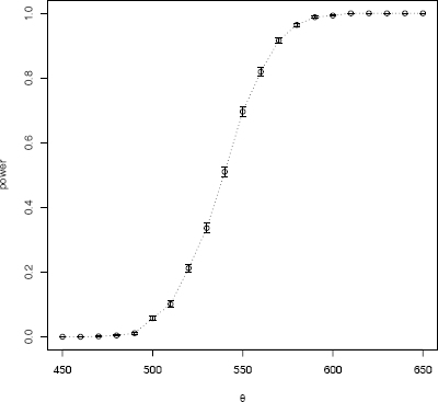
Use simulation to estimate power and plot an empirical power curve for the t-test in Example 6.7. (For a numerical approach that does not involve simulation, see the remark below.)
To plot the curve, we need the empirical power for a sequence of alternatives θ along the horizontal axis. Each point corresponds to a Monte Carlo experiment. The outer for loop varies the points θ (mu) and the inner replicate loop (see R Note 6.1) estimates the power at the current θ.
n <- 20
m <- 1000
mu0 <- 500
sigma <- 100
mu <- c(seq(450, 650, 10)) #alternatives
M <- length(mu)
power <- numeric(M)
for (i in 1:M) {
mu1 <- mu[i]
pvalues <- replicate(m, expr = {
#simulate under alternative mu1
x <- rnorm(n, mean = mu1, sd = sigma)
ttest <- t.test(x,
alternative = "greater", mu = mu0)
ttest$p.value})
power[i] <- mean(pvalues <= .05)
}
The estimated power values are now stored in the vector power. Next, plot the empirical power curve, adding vertical error bars at using the errbar function in the Hmisc package [132].
library(Hmisc) #for errbar
plot(mu, power)
abline(v = mu0, lty = 1)
abline(h = .05, lty = 1)
#add standard errors
se <- sqrt(power * (1-power) / m)
errbar(mu, power, yplus = power+se, yminus = power-se,
xlab = bquote(theta))
lines(mu, power, lty=3)
detach(package:Hmisc)
The power curve is shown in Figure 6.1. Note that the empirical power is small when θ is close to θ0 = 500, and increasing as θ moves farther away from θ0, approaching 1 as θ → ∞.
Remark 6.2
The non-central t distribution arises in power calculations for t-tests. The general non-central t with parameters (ν, δ) is defined as the distribution of where Z ~ N (0,1) and V ~ x2(ν) are independent.
Suppose X1, X2, ... , Xn is a random sample from a N(μ, σ2) distribution, and the t-statistic is applied to test H0 : μ = μ0. Under the null hypothesis, T has the central t(n−1) distribution, but if μ ≠ μ0, T has the non-central t distribution with n − 1 degrees of freedom and non-centrality parameter A numerical approach to evaluating the cdf of the non-central t distribution, based on an algorithm of Lenth [175], is implemented in the R function pt. Also see power.t.test.
Example 6.10 (Power of the skewness test of normality)
The skewness test of normality was described in Example 6.8. In this example, we estimate by simulation the power of the skewness test of normality against a contaminated normal (normal scale mixture) alternative described in Example 6.3. The contaminated normal distribution is denoted by
When ε = 0 or ε = 1 the distribution is normal, but the mixture is non-normal for 0 ε 1. We can estimate the power of the skewness test for a sequence of alternatives indexed by ε and plot a power curve for the power of the skewness test against this type of alternative. For this experiment, the significance level is α = 0.1 and the sample size is n = 30. The skewness statistic sk is implemented in Example 6.8.
alpha <- .1
n <- 30
m <- 2500
epsilon <- c(seq(0, .15, .01), seq(.15, 1, .05))
N <- length(epsilon)
pwr <- numeric(N)
#critical value for the skewness test
cv <- qnorm(1-alpha/2, 0, sqrt(6*(n-2) / ((n+1)*(n+3))))
for (j in 1:N) { #for each epsilon
e <- epsilon[j]
sktests <- numeric(m)
for (i in 1:m) { #for each replicate
sigma <- sample(c(1, 10), replace = TRUE,
size = n, prob = c(1-e, e))
x <- rnorm(n, 0, sigma)
sktests[i] <- as.integer(abs(sk(x)) >= cv)
}
pwr[j] <- mean(sktests)
}
#plot power vs epsilon
plot(epsilon, pwr, type = "b",
xlab = bquote(epsilon), ylim = c(0,1))
abline(h = .1, lty = 3)
se <- sqrt(pwr * (1-pwr) / m) #add standard errors
lines(epsilon, pwr+se, lty = 3)
lines(epsilon, pwr-se, lty = 3)
The empirical power curve is shown in Figure 6.2. Note that the power curve crosses the horizontal line corresponding to α = 0.10 at both endpoints, ε = 0 and ε = 1 where the alternative is normally distributed. For 0 < ε < 1 the empirical power of the test is greater than 0.10 and highest when ε is about 0.15.
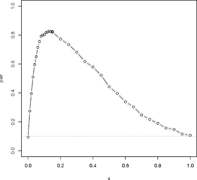
Empirical power for the skewness test of normality against ∈contaminated normal scale mixture alternative in Example 6.10.
6.3.3 Power comparisons
Monte Carlo methods are often applied to compare the performance of different test procedures. A skewness test of normality was introduced in Example 6.8. There are many tests of normality in the literature (see [58] and [270]). In the following example three tests of univariate normality are compared.
Example 6.11 (Power comparison of tests of normality)
Compare the empirical power of the skewness test of univariate normality with the Shapiro-Wilk [248] test. Also compare the power of the energy test [263], which is based on distances between sample elements.
Let denote the family of univariate normal distributions. Then the test hypotheses are
The Shapiro-Wilk test is based on the regression of the sample order statistics on their expected values under normality, so it falls in the general category of tests based on regression and correlation. The approximate critical values of the statistic are determined by a transformation of the statistic W to normality [235, 236, 237] for sample sizes 7 ≤ n ≤ 2000. The Shapiro-Wilk test is implemented by the R function shapiro.test.
The energy test is based on an energy distance between the sampled distribution and normal distribution, so large values of the statistic are significant. The energy test is a test of multivariate normality [263], so the test considered here is the special case d = 1. As a test of univariate normality, energy performs very much like the Anderson-Darling test [9]. The energy statistic for testing normality is
where X, X′ are iid. Large values of Qn are significant. In the univariate case, the following computing formula is equivalent:
where , Y(k) is the kth order statistic of the standardized sample, Φ is the standard normal cdf and ϕ is the standard normal density. If the parameters are unknown, substitute the sample mean and sample standard deviation to to compute Y1, ... , Yn. A computing formula for the multivariate case is given in [263]. The energy test for univariate and multivariate normality is implemented in mvnorm.etest in the energy package [226].
The skewness test of normality was introduced in Examples 6.8 and 6.10. The sample skewness function sk is given in Example 6.8 on page 166.
For this comparison we set significance level α = 0.1. The example below compares the power of the tests against the contaminated normal alternatives described in Example 6.3. The alternative is the normal mixture denoted by
When ε = 0 or ε = 1 the distribution is normal, and in this case the empirical Type I error rate should be controlled at approximately the nominal rate α = 0.1. If 0 < ε < 1 the distributions are non-normal, and we are interested in comparing the empirical power of the tests against these alternatives.
# initialize input and output
library(energy)
alpha <- .1
n <- 30
m <- 2500 #try smaller m for a trial run
epsilon <- .1
test1 <- test2 <- test3 <- numeric(m)
#critical value for the skewness test
cv <- qnorm(1-alpha/2, 0, sqrt(6*(n-2) / ((n+1)*(n+3))))
# estimate power
for (j in 1:m) {
e <- epsilon
sigma <- sample(c(1, 10), replace = TRUE,
size = n, prob = c(1-e, e))
x <- rnorm(n, 0, sigma)
test1[j] <- as.integer(abs(sk(x)) >= cv)
test2[j] <- as.integer(
shapiro.test(x)$p.value <= alpha)
test3[j] <- as.integer(
mvnorm.etest(x, R=200)$p.value <= alpha)
}
print(c(epsilon, mean(test1), mean(test2), mean(test3)))
detach(package:energy)
The simulation was repeated for several choices of ε and results saved in a matrix sim. Simulation results for n = 30 are summarized in Table 6.2 and in Figure 6.3. The plot is obtained as follows.
Empirical Power of Three Tests of Normality against a Contaminated Normal Alternative in Example 6.11 (n = 30, α = 0.1, se ≤ 0.01)
ε |
skewness test |
Shapiro-Wilk |
energy test |
|---|---|---|---|
0.00 |
0.0984 |
0.1076 |
0.1064 |
0.05 |
0.6484 |
0.6704 |
0.6560 |
0.10 |
0.8172 |
0.9008 |
0.8896 |
0.15 |
0.8236 |
0.9644 |
0.9624 |
0.20 |
0.7816 |
0.9816 |
0.9800 |
0.25 |
0.7444 |
0.9940 |
0.9924 |
0.30 |
0.6724 |
0.9960 |
0.9980 |
0.40 |
0.5672 |
0.9828 |
0.9964 |
0.50 |
0.4424 |
0.9112 |
0.9724 |
0.60 |
0.3368 |
0.7380 |
0.8868 |
0.70 |
0.2532 |
0.4900 |
0.6596 |
0.80 |
0.1980 |
0.2856 |
0.3932 |
0.90 |
0.1296 |
0.1416 |
0.1724 |
1.00 |
0.0992 |
0.0964 |
0.0980 |
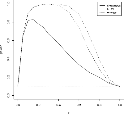
Empirical power of three tests of normality against a contaminated normal alternative in Example 6.11 (n = 30, α = 0.1, se ≤ 0.01)
# plot the empirical estimates of power
plot(sim[,1], sim[,2], ylim = c(0, 1), type = "l",
xlab = bquote(epsilon), ylab = "power")
lines(sim[,1], sim[,3], lty = 2)
lines(sim[,1], sim[,4], lty = 4)
abline(h = alpha, lty = 3)
legend("topright", 1, c("skewness", "S-W", "energy"),
lty = c(1,2,4), inset = .02)
Standard error of the estimates is at most Estimates for empirical Type I error rate correspond to ε = 0 and ε = 1. All tests achieve approximately the nominal significance level α = 0.10 within one standard error. The tests are at approximately the same significance level, so it is meaningful to compare the results for power.
The simulation results suggest that the Shapiro-Wilk and energy tests are about equally powerful against this type of alternative when n = 30 and ε < 0.5. Both have higher power than the skewness test overall and energy appears to have highest power for 0.5 ≤ ε ≤ 0.8.
6.4 Application: “Count Five” Test for Equal Variance
The examples in this section illustrate the Monte Carlo method for a simple two sample test of equal variance.
The two sample “Count Five” test for equality of variance introduced by McGrath and Yeh [193] counts the number of extreme points of each sample relative to the range of the other sample. Suppose the means of the two samples are equal and the sample sizes are equal. An observation in one sample is considered extreme if it is not within the range of the other sample. If either sample has five or more extreme points, the hypothesis of equal variance is rejected.
Example 6.12 (Count Five test statistic)
The computation of the test statistic is illustrated with a numerical example. Compare the side-by-side boxplots in Figure 6.4 and observe that there are some extreme points in each sample with respect to the other sample.
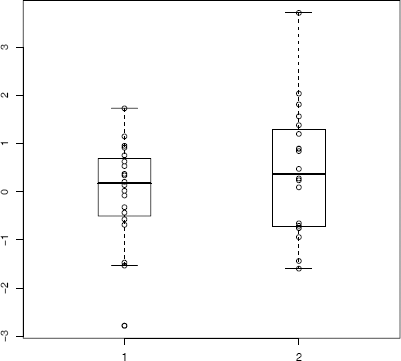
x1 <- rnorm(20, 0, sd = 1)
x2 <- rnorm(20, 0, sd = 1.5)
y <- c(x1, x2)
group <- rep(1:2, each = length(x1))
boxplot(y ~ group, boxwex = .3, xlim = c(.5, 2.5), main = "")
points(group, y)
# now identify the extreme points
> range(x1)
[1] -2.782576 1.728505
> range(x2)
[1] -1.598917 3.710319
> i <- which(x1 < min(x2))
> j <- which(x2 > max(x1))
> x1[i]
[1] -2.782576
> x2[j]
[1] 2.035521 1.809902 3.710319
The Count Five statistic is the maximum number of extreme points, max(1, 3), so the Count Five test will not reject the hypothesis of equal variance. Note that we only need the number of extreme points, and the extreme count can be determined without reference to a boxplot as follows.
out1 <- sum(x1 > max(x2)) + sum(x1 < min(x2))
out2 <- sum(x2 > max(x1)) + sum(x2 < min(x1))
> max(c(out1, out2))
[1] 3
Example 6.13 (Count Five test statistic, cont.)
Consider the case of two independent random samples from the same normal distribution. Estimate the sampling distribution of the maximum number of extreme points, and find the 0.80, 0.90, and 0.95 quantiles of the sampling distribution.
The function maxout below counts the maximum number of extreme points of each sample with respect to the range of the other sample. The sampling distribution of the extreme count statistic can be estimated by a Monte Carlo experiment.
maxout <- function(x, y) {
X <- x − mean(x)
Y <- y − mean(y)
outx <- sum(X > max(Y)) + sum(X < min(Y))
outy <- sum(Y > max(X)) + sum(Y < min(X))
return(max(c(outx, outy)))
}
n1 <- n2 <- 20
mu1 <- mu2 <- 0
sigma1 <- sigma2 <- 1
m <- 1000
# generate samples under H0
stat <- replicate(m, expr={
x <- rnorm(n1, mu1, sigma1)
y <- rnorm(n2, mu2, sigma2)
maxout(x, y)
})
print(cumsum(table(stat)) / m)
print(quantile(stat, c(.8, .9, .95)))
The “Count Five” test criterion looks reasonable for normal distributions. The empirical cdf and quantiles are
1 2 3 4 5 6 7 8 9 10 11
0.149 0.512 0.748 0.871 0.945 0.974 0.986 0.990 0.996 0.999 1.000
80% 90% 95%
4 5 6
Notice that the quantile function gives 6 as the 0.95 quantile. However, if α = 0.05 is the desired significance level, the critical value 5 appears to be the best choice. The quantile function is not always the best way to estimate a critical value. If quantile is used, compare the result to the empirical cdf.
The “Count Five” test criterion can be applied for independent random samples when the random variables are similarly distributed and sample sizes are equal. (Random variables X and Y are called similarly distributed if Y has the same distribution as (X − a)/b where a and b > 0 are constants.) When the data are centered by their respective population means, McGrath and Yeh [193] show that the Count Five test on the centered data has significance level at most 0.0625.
In practice, the populations means are generally unknown and each sample would be centered by subtracting its sample mean. Also, the sample sizes may be unequal.
Example 6.14 (Count Five test)
Use Monte Carlo methods to estimate the significance level of the test when each sample is centered by subtracting its sample mean. Here again we consider normal distributions. The function count5test returns the value 1 (reject H0) or 0 (do not reject H0).
count5test <- function(x, y) {
X <- x − mean(x)
Y <- y − mean(y)
outx <- sum(X > max(Y)) + sum(X < min(Y))
outy <- sum(Y > max(X)) + sum(Y < min(X))
# return 1 (reject) or 0 (do not reject H0)
return(as.integer(max(c(outx, outy)) > 5))
}
n1 <- n2 <- 20
mu1 <- mu2 <- 0
sigma1 <- sigma2 <- 1
m <- 10000
tests <- replicate(m, expr = {
x <- rnorm(n1, mu1, sigma1)
y <- rnorm(n2, mu2, sigma2)
x <- x − mean(x) #centered by sample mean
y <- y − mean(y)
count5test(x, y)
})
alphahat <- mean(tests)
> print(alphahat)
[1] 0.0565
If the samples are centered by the population mean, we should expect an empirical Type I error rate of about 0.055, from our previous simulation to estimate the quantiles of the maxout statistic. In the simulation, each sample was centered by subtracting the sample mean, and the empirical Type I error rate was 0.0565 (se ≐ 0.0022).
Example 6.15 (Count Five test, cont.)
Repeating the previous example, we are estimating the empirical Type I error rate when sample sizes differ and the “Count Five” test criterion is applied. Each sample is centered by subtracting the sample mean.
n1 <- 20
n2 <- 30
mu1 <- mu2 <- 0
sigma1 <- sigma2 <- 1
m <- 10000
alphahat <- mean(replicate(m, expr={
x <- rnorm(n1, mu1, sigma1)
y <- rnorm(n2, mu2, sigma2)
x <- x − mean(x) #centered by sample mean
y <- y − mean(y)
count5test(x, y)}))
print(alphahat)
[1] 0.1064
The simulation result suggests that the “Count Five” criterion does not necessarily control Type I error at α ≤ 0.0625 when the sample sizes are unequal. Repeating the simulation above with n1 = 20 and n2 = 50, the empirical Type I error rate was 0.2934. See [193] for a method to adjust the test criterion for unequal sample sizes.
Example 6.16 (Count Five, cont.)
Use Monte Carlo methods to estimate the power of the Count Five test, where the sampled distributions are , and the sample sizes are n1 = n2 = 20.
# generate samples under H1 to estimate power
sigma1 <- 1
sigma2 <- 1.5
power <- mean(replicate(m, expr={
x <- rnorm(20, 0, sigma1)
y <- rnorm(20, 0, sigma2)
count5test(x, y)
}))
> print(power)
[1] 0.3129
The empirical power of the test is 0.3129 (se ≤ 0.005) against the alternative (σ1 = 1, σ2 = 1.5) with n1 = n2 = 20. See [193] for power comparisons with other tests for equal variance and applications.
Exercises
6.1 Estimate the MSE of the level k trimmed means for random samples of size 20 generated from a standard Cauchy distribution. (The target parameter θ is the center or median; the expected value does not exist.) Summarize the estimates of MSE in a table for k = 1, 2, ... , 9.
6.2 Plot the empirical power curve for the t-test in Example 6.9, changing the alternative hypothesis to H1 : μ ≠ 500, and keeping the significance level α = 0.05.
6.3 Plot the power curves for the t-test in Example 6.9 for sample sizes 10, 20, 30, 40, and 50, but omit the standard error bars. Plot the curves on the same graph, each in a different color or different line type, and include a legend. Comment on the relation between power and sample size.
6.4 Suppose that X1, ..., Xn are a random sample from a from a lognormal distribution with unknown parameters. Construct a 95% confidence interval for the parameter μ. Use a Monte Carlo method to obtain an empirical estimate of the confidence level.
6.5 Suppose a 95% symmetric t-interval is applied to estimate a mean, but the sample data are non-normal. Then the probability that the confidence interval covers the mean is not necessarily equal to 0.95. Use a Monte Carlo experiment to estimate the coverage probability of the t-interval for random samples of x2(2) data with sample size n = 20. Compare your t-interval results with the simulation results in Example 6.4. (The t-interval should be more robust to departures from normality than the interval for variance.)
6.6 Estimate the 0.025, 0.05, 0.95, and 0.975 quantiles of the skewness under normality by a Monte Carlo experiment. Compute the standard error of the estimates from (2.14) using the normal approximation for the density (with exact variance formula). Compare the estimated quantiles with the quantiles of the large sample approximation
6.7 Estimate the power of the skewness test of normality against symmetric Beta(α, α) distributions and comment on the results. Are the results different for heavy-tailed symmetric alternatives such as t(ν)?
6.8 Refer to Example 6.16. Repeat the simulation, but also compute the F test of equal variance, at significance level Compare the power of the Count Five test and F test for small, medium, and large sample sizes. (Recall that the F test is not applicable for non-normal distributions.)
6.9 Let X be a non-negative random variable with μ = E[X] < ∞. For a random sample x1, ... , xn from the distribution of X, the Gini ratio is defined by
The Gini ratio is applied in economics to measure inequality in income distribution (see e.g. [163]). Note that G can be written in terms of the order statistics x(i) as
If the mean is unknown, let be the statistic G with μ replaced by . Estimate by simulation the mean, median and deciles of if X is standard lognormal. Repeat the procedure for the uniform distribution and Bernoulli(0.1). Also construct density histograms of the replicates in each case.
6.10 Construct an approximate 95% confidence interval for the Gini ratio γ = E[G] if X is lognormal with unknown parameters. Assess the coverage rate of the estimation procedure with a Monte Carlo experiment.
Projects
6.A Use Monte Carlo simulation to investigate whether the empirical Type I error rate of the t-test is approximately equal to the nominal significance level α, when the sampled population is non-normal. The t-test is robust to mild departures from normality. Discuss the simulation results for the cases where the sampled population is (i) χ2(1), (ii) Uniform(0,2), and (iii) Exponential(rate=1). In each case, test H0 : μ = μ0 vs H0 : μ ≠ μ0, where μ0 is the mean of χ2(1), Uniform(0,2), and Exponential(1), respectively.
6.B Tests for association based on Pearson product moment correlation ρ, Spearman’s rank correlation coefficient ρs, or Kendall’s coefficient τ, are implemented in cor.test. Show (empirically) that the nonparametric tests based on ρs or τ are less powerful than the correlation test when the sampled distribution is bivariate normal. Find an example of an alternative (a bivariate distribution (X, Y) such that X and Y are dependent) such that at least one of the nonparametric tests have better empirical power than the correlation test against this alternative.
6.C Repeat Examples 6.8 and 6.10 for Mardia’s multivariate skewness test. Mardia [187] proposed tests of multivariate normality based on multivariate generalizations of skewness and kurtosis. If X and Y are iid, the multivariate population skewness is defined by Mardia as
Under normality, The multivariate skewness statistic is
where is the maximum likelihood estimator of covariance. Large values of b1,d are significant. The asymptotic distribution of is chisquared with d(d + 1)(d + 2)/6 degrees of freedom.
6.D Repeat Example 6.11 for multivariate tests of normality. Mardia [187] defines multivariate kurtosis as
For d-dimensional multivariate normal distributions the kurtosis coefficient is β2,d = d(d + 2). The multivariate kurtosis statistic is
The large sample test of multivariate normality based on b2,d rejects the null hypothesis at significance level α if
However, b2,d converges very slowly to the normal limiting distribution. Compare the empirical power of Mardia’s skewness and kurtosis tests of multivariate normality with the energy test of multivariate normality mvnorm.etest(energy) (6.3) [226, 263]. Consider multivariate normal location mixture alternatives where the two samples are generated from mlbench.twonorm in the mlbench package [174].