
Methods for Generating Random Variables
3.1 Introduction
One of the fundamental tools required in computational statistics is the ability to simulate random variables from specified probability distributions. On this topic many excellent references are available. On the general subject of methods for generating random variates from specified probability distributions, readers are referred to [69, 94, 112, 114, 154, 228, 223, 233, 238]. On specific topics, also see [3, 4, 31, 43, 68, 98, 155, 159, 190].
In the simplest case, to simulate drawing an observation at random from a finite population, a method of generating random observations from the discrete uniform distribution is required. Therefore a suitable generator of uniform pseudo random numbers is essential. Methods for generating random variates from other probability distributions all depend on the uniform random number generator.
In this text we assume that a suitable uniform pseudo random number generator is available. Refer to the help topic for .Random.seed or RNGkind for details about the default random number generator in R. For reference about different types of random number generators and their properties see Gentle [112] and Knuth [164].
The uniform pseudo random number generator in R is runif. To generate a vector of n (pseudo) random numbers between 0 and 1 use runif(n). Throughout this text, whenever computer generated random numbers are mentioned, it is understood that these are pseudo random numbers. To generate n random Uniform(a, b) numbers use runif(n, a, b). To generate an n by m matrix of random numbers between 0 and 1 use matrix(runif(n*m), nrow=n, ncol=m) or matrix(runif(n*m), n, m).
In the examples of this chapter, several functions are given for generating random variates from continuous and discrete probability distributions. Generators for many of these distributions are available in R (e.g. rbeta, rgeom, rchisq, etc.), but the methods presented below are general and apply to many other types of distributions. These methods are also applicable for external libraries, stand alone programs, or nonstandard simulation problems.
Most of the examples include a comparison of the generated sample with the theoretical distribution of the sampled population. In some examples, histograms, density curves, or QQ plots are constructed. In other examples summary statistics such as sample moments, sample percentiles, or the empirical distribution are compared with the corresponding theoretical values. These are informal approaches to check the implementation of an algorithm for simulating a random variable.
Example 3.1 (Sampling from a finite population)
The sample function can be used to sample from a finite population, with or without replacement.
> #toss some coins
> sample(0:1, size = 10, replace = TRUE)
[1] 0 1 1 1 0 1 1 1 1 0
> #choose some lottery numbers
> sample(1:100, size = 6, replace = FALSE)
[1] 51 89 26 99 74 73
> #permuation of letters a-z
> sample(letters)
[1] "d" "n" "k" "x" "s" "p" "j" "t" "e" "b" "g"
"a" "m" "y" "i" "v" "l" "r" "w" "q" "z"
[22] "u" "h" "c" "f" "o"
> #sample from a multinomial distribution
> x <- sample(1:3, size = 100, replace = TRUE,
prob = c(.2, .3, .5))
> table(x)
x
1 2 3
17 35 48
Random Generators of Common Probability Distributions in R
In the sections that follow, various methods of generating random variates from specified probability distributions are presented. Before discussing those methods, however, it is useful to summarize some of the probability functions available in R. The probability mass function (pmf) or density (pdf), cumulative distribution function (cdf), quantile function, and random generator of many commonly used probability distributions are available. For example, four functions are documented in the help topic Binomial:
dbinom(x, size, prob, log = FALSE)
pbinom(q, size, prob, lower.tail = TRUE, log.p = FALSE)
qbinom(p, size, prob, lower.tail = TRUE, log.p = FALSE)
rbinom(n, size, prob)
The same pattern is applied to other probability distributions. In each case, the abbreviation for the name of the distribution is combined with first letter d for density or pmf, p for cdf, q for quantile, or r for random generation from the distribution.
A partial list of available probability distributions and parameters is given in Table 3.1. For a complete list, refer to the R documentation [279, Ch. 8]. In addition to the parameters listed, some of the functions take optional log, lower.tail, or log.p arguments, and some take an optional ncp (noncentrality) parameter.
Selected Univariate Probability Functions Available in R
Distribution |
cdf |
Generator |
Parameters |
|---|---|---|---|
beta |
pbeta |
rbeta |
shape1,shape2 |
binomial |
pbinom |
rbinom |
size,prob |
chi-squared |
pchisq |
rchisq |
df |
exponential |
pexp |
rexp |
rate |
F |
pf |
rf |
df1, df2 |
gaama |
pgaama |
rgaama |
shape, rate or scale |
geometric |
pgeom |
rgeom |
prob |
lognormal |
plnorm |
rlnorm |
meanlog,sdlog |
negative binomial |
pnbinom |
rnbinom |
size,prob |
normal |
pnorm |
rnorm |
mean, sd |
poisson |
ppois |
rpois |
lambda |
stubents t |
pt |
rt |
df |
uniform |
punif |
runif |
min,max |
3.2 The Inverse Transform Method
The inverse transform method of generating random variables is based on the following well known result (see e.g. [16, p. 201] or [231, p. 203]).
THEOREM 3.1 (Probability Integral Transformation)
If X is a continuous random variable with cdf FX(x), then U=FX(X)~ uniform(0,1).
The inverse transform method of generating random variables applies the probability integral transformation. Define the inverse transformation
F−1X(u)=inf{x:FX(x)=u}, 0<u<1.
If U ~ Uniform(0, 1), then for all x∈ℝ
P(F−1X(U)≤x)=P(inf{t: FX(t)=U}≤x) =P(U≤FX(x)) =FU(FX(x))=FX(x),
and therefore F−1X(U) has the same distribution as X. Thus, to generate a random observation X, first generate a Uniform(0,1) variate u and deliver the inverse value F−1X(u). The method is easy to apply, provided that F−1X is easy to compute. The method can be applied for generating continuous or discrete random variables. The method can be summarized as follows.
- Derive the inverse function F−1X(u).
- Write a command or function to compute F−1X(u).
- For each random variate required:
- Generate a random u from Uniform(0,1).
- Deliver x=F−1X(u)
3.2.1 Inverse Transform Method, Continuous Case
Example 3.2 (Inverse transform method, continuous case)
This example uses the inverse transform method to simulate a random sample from the distribution with density fX(x), = 3x2, 0 < x <1.
Here FX(x)=x3 for 0 < x < 1, and F−1X(u)=u13. Generate all n required random uniform numbers as vector u. Then uˆ(1/3) is a vector of length n containing the sample x1,..., xn.
n <- 1000
u <- runif(n)
x <- uˆ(1/3)
hist(x, prob = TRUE) #density histogram of sample
y <- seq(0, 1, .01)
lines(y, 3*yˆ2) #density curve f(x)
The histogram and density plot in Figure 3.1 suggests that the empirical and theoretical distributions approximately agree.
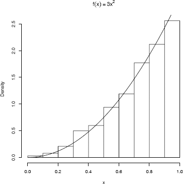
Probability density histogram of a random samplegenerated by the inverse transform method in Example 3.2, with the theoretical density f(x) = 3x2 superimposed.
R note 3.1 In Figure 3.1, the title includes a math expression. This title is obtained by specifying the main title using the expression function as follows:
hist(x, prob = TRUE, main = expression(f(x)==3*x^2))
Alternately, main = bquote(f(x)==3*x^2)) produces the same title. Math annotation is covered in the help topic for plotmath. Also see the help topics for text and axis.
Example 3.3 (Exponential distribution)
This example applies the inverse transform method to generate a random sample from the exponential distribution with mean 1/λ.
If X ~ Exp(λ), then for x > 0 the cdf of X is FX(x)=1−e−λx. The inverse transformation is F−1X(u)=−1λlog(1−u). Note that U and 1 − U have the same distribution and it is simpler to set x=−1λlog(u). To generate a random sample of size n with parameter lambda:
-log(runif(n)) / lambda
A generator rexp is available in R. However, this algorithm is very useful for implementation in other situations, such as a C program.
3.2.2 Inverse Transform Method, Discrete Case
The inverse transform method can also be applied to discrete distributions. If X is a discrete random variable and
...<xi−1 <xi<xi+1<...
are the points of discontinuity of FX(x), then the inverse transformation is F−1X(u)=xi, where FX(xi−1)<u≤FX(xi)
For each random variate required:
- Generate a random u from Uniform(0,1).
- Deliver xi where F(xi−1)<u≤F(xi)
The solution of F(xi−1)<u≤F(xi) in Step (2) may be difficult for some distributions. See Devroye [69, Ch. III] for several different methods of implementing the inverse transform method in the discrete case.
Example 3.4 (Two point distribution)
This example applies the inverse transform to generate a random sample of Bernoulli(p = 0.4) variates. Although there are simpler methods to generate a two point distribution in R, this example illustrates computing the inverse cdf of a discrete random variable in the simplest case.
In this example, FX(0) = fX(0)= 1-p and FX(1) = 1. Thus F−1X(u)=1 if u > 0.6 and F−1X(u)=0 if u ≤ 0.6. The generator should therefore deliver the numerical value of the logical expression u > 0.6.
n <- 1000
p <- 0.4
u <- runif(n)
x <- as.integer(u > 0.6) #(u > 0.6) is a logical vector
> mean(x)
[1] 0.41
> var(x)
[1] 0.2421421
Compare the sample statistics with the theoretical moments. The sample mean of a generated sample should be approximately p = 0.4 and the sample variance should be approximately p(1 − p) = 0.24. Our sample statistics are ˉx=0.41 (se=√0.241000=0.0155) and s2=0.242.
R note 3.2 In R one can use the rbinom (random binomial) function with size=1 to generate a Bernoulli sample. Another method is to sample from the vector (0,1) with probabilities (1 − p, p).
rbinom(n, size = 1, prob = p)
sample(c(0,1), size = n, replace = TRUE, prob = c(.6,.4))
Also see Example 3.1.
Example 3.5 (Geometric distribution)
Use the inverse transform method to generate a random geometric sample with parameter p = 1/4.
The pmf is f(x) = pqx, x = 0, 1, 2, ... , where q = 1 − p. At the points of discontinuity x = 0, 1, 2, ...,the cdf is F(x) = 1 − qx+1. For each sample element we need to generate a random uniform u and solve
1−qx<u≤1−qx+1.
This inequality simplifies to x<log(1−u)log(q)≤x+1. The solution is x+1=⌈log(1−u)log(q)⌉ where ⌈t⌉ denotes the ceiling function (the smallest integer not less than t).
n <- 1000
p <- 0.25
u <- runif(n)
k <- ceiling(log(1-u) / log(1-p)) - 1
Here again there is a simplification, because U and 1 − U have the same distribution. Also, the probability that log(1−u)log(1−p) equals an integer is zero. The last step can therefore be simplified to
k <- floor(log(u) / log(1-p))
The geometric distribution was particularly easy to simulate by the inverse transform method because it was easy to solve the inequality
F(x−1)<u≤F(x)
rather than compare each u to all the possible values F(x). The same method applied to the Poisson distribution is more complicated because we do not have an explicit formula for the value of x such that F(x − 1) < u ≤ F(x).
The R function rpois generates random Poisson samples. The basic method to generate a Poisson(λ) variate (see e.g. [233]) is to generate and store the cdf via the recursive formula
f(x+1)=λf(x)x+1; F(x+1)=F(x)+f(x+1).
For each Poisson variate required, a random uniform u is generated, and the cdf vector is searched for the solution to F(x − 1) < u ≤ F(x).
To illustrate the main idea of the inverse transform method for generating Poisson variates, here is a similar example for which there is no R generator available: the logarithmic distribution. The logarithmic distribution is a one parameter discrete distribution supported on the positive integers.
Example 3.6 (Logarithmic distribution)
This example implements a function to simulate a Logarithmic(θ) random sample by the inverse transform method. A random variable X has the logarithmic distribution (see [158], Ch. 7) if
f(x)=p(X=x)=aθxx, x=1,2,... (3.1)
where 0 < θ < 1 and a=(−log(1−θ))−1. A recursive formula for f(x) is
f(x+1)=θzx+1f(x), x=1,2,.... (3.2)
Theoretically, the pmf can be evaluated recursively using (3.2), but the calculation is not sufficiently accurate for large values of x and ultimately produces f(x) = 0 with F(x) < 1. Instead we compute the pmf from (3.1) as exp(log a + x log θ − log x). In generating a large sample, there will be many repetitive calculations of the same values F(x). It is more efficient to store the cdf values. Initially choose a length N for the cdf vector, and compute F(x), x = 1, 2, ... , N. If necessary, N will be increased.
To solve F(x−1) < u ≤ F(x) for a particular u, it is necessary to count the number of values x such that F(x −1) < u. If F is a vector and ui is a scalar, then the expression F < ui produces a logical vector; that is, a vector the same length as F containing logical values TRUE or FALSE. In an arithmetic expression, TRUE has value 1 and FALSE has value 0. Notice that the sum of the logical vector (ui > F) is exactly x − 1.
The code for logarithmic is on the next page. Generate random samples from a Logarithmic(0.5) distribution.
n <- 1000
theta <- 0.5
x <- rlogarithmic(n, theta)
#compute density of logarithmic(theta) for comparison
k <- sort(unique(x))
p <- -1 / log(1 - theta) * theta^k / k
se <- sqrt(p*(1-p)/n) #standard error
In the following results, the relative frequencies of the sample (first line) match the theoretical distribution (second line) of the Logarithmic(0.5) distribution within two standard errors.
> round(rbind(table(x)/n, p, se),3)
1 2 3 4 5 6 7
0.741 0.169 0.049 0.026 0.008 0.003 0.004
p 0.721 0.180 0.060 0.023 0.009 0.004 0.002
se 0.014 0.012 0.008 0.005 0.003 0.002 0.001
rlogarithmic <- function(n, theta) {
#returns a random logarithmic(theta) sample size n
u <- runif(n)
#set the initial length of cdf vector
N <- ceiling(-16 / log10(theta))
k <- 1:N
a <- -1/log(1-theta)
fk <- exp(log(a) + k * log(theta) - log(k))
Fk <- cumsum(fk)
x <- integer(n)
for (i in 1:n) {
x[i] <- as.integer(sum(u[i] > Fk)) #F^{-1}(u)-1
while (x[i] == N) {
#if x==N we need to extend the cdf
#very unlikely because N is large
logf <- log(a) + (N+1)*log(theta) - log(N+1)
fk <- c(fk, exp(logf))
Fk <- c(Fk, Fk[N] + fk[N+1])
N <- N + 1
x[i] <- as.integer(sum(u[i] > Fk))
}
}
x + 1
}
Remark 3.1
A more efficient generator for the Logarithmic(θ) distribution is implemented in Example 3.9 of Section 3.4.
3.3 The Acceptance-Rejection Method
Suppose that X and Y are random variables with density or pmf f and g respectively, and there exists a constant c such that
f(t)g(t)≤c
for all t such that f(t) > 0. Then the acceptance-rejection method (or rejection method) can be applied to generate the random variable X.
The Acceptance-Rejection Method
- Find a random variable Y with density g satisfying f(t)/g(t) ≤ c, for all t such that f(t) > 0. Provide a method to generate random Y.
- For each random variate required:
- Generate a random y from the distribution with density g.
- Generate a random u from the Uniform(0, 1) distribution.
- If u < f(y)/(cg(y)) accept y and deliver x = y; otherwise reject y and repeat from step (2a).
Note that in step (2c),
p(accept|Y)=p(U<f(Y)cg(Y)|Y)=f(Y)cg(Y).
The last equality is simply evaluating the cdf of U. The total probability of acceptance for any iteration is therefore
∑yp(accept|y)P(Y=y)=∑yf(y)cg(y)g(y)=1c,
and the number of iterations until acceptance has the geometric distribution with mean c. Hence, on average each sample value of X requires c iterations. For efficiency, Y should be easy to simulate and c small.
To see that the accepted sample has the same distribution as X, apply Bayes’ Theorem. In the discrete case, for each k such that f(k) > 0,
P(k|accepted)=p(accepted|k)g(k)p(accepted)=[f(k)(cg(k))]g(k)1c=f(k).
The continuous case is similar.
Example 3.7 (Acceptance-rejection method)
This example illustrates the acceptance-rejection method for the beta distribution. On average, how many random numbers must be simulated to generate 1000 variates from the Beta(α = 2, β = 2) distribution by this method? It depends on the upper bound c of f(x)/g(x), which depends on the choice of the function g(x).
The Beta(2,2) density is f(x) = 6x(1 − x), 0 < x < 1. Let g(x) be the Uniform(0,1) density. Then f(x)g(x)≤6 for all 0 < x< 1, so c = 6. A random x from g(x) is accepted if
f(x)cg(x)=6x(1−x)6(1)=x(1−x)>u.
On average, cn = 6000 iterations (12000 random numbers) will be required for a sample size 1000. In the following simulation, the counter j for iterations is not necessary, but included to record how many iterations were actually needed to generate the 1000 beta variates.
n <- 1000
k <- 0 #counter for accepted
j <- 0 #iterations
y <- numeric(n)
while (k < n) {
u <- runif(1)
j <- j + 1
x <- runif(1) #random variate from g
if (x * (1-x) > u) {
#we accept x
k <- k + 1
y[k] <- x
}
}
> j
[1] 5873
In this simulation, 5873 iterations (11746 random numbers) were required to generate the 1000 beta variates. Compare the empirical and theoretical percentiles.
#compare empirical and theoretical percentiles
p <- seq(.1, .9, .1)
Qhat <- quantile(y, p) #quantiles of sample
Q <- qbeta(p, 2, 2) #theoretical quantiles
se <- sqrt(p * (1-p) / (n * dbeta(Q, 2, 2))) #see Ch. 1
The sample percentiles (first line) approximately match the Beta(2,2) percentiles computed by qbeta (second line), most closely near the center of the distribution. Larger numbers of replicates are required for estimation of percentiles where the density is close to zero.
> round(rbind(Qhat, Q, se), 3)
10% 20% 30% 40% 50% 60% 70% 80% 90%
Qhat 0.189 0.293 0.365 0.449 0.519 0.589 0.665 0.741 0.830
Q 0.196 0.287 0.363 0.433 0.500 0.567 0.637 0.713 0.804
se 0.010 0.011 0.012 0.013 0.013 0.013 0.012 0.011 0.010
Repeating the simulation with n = 10000 produces more precise estimates.
> round(rbind(Qhat, Q, se), 3)
10% 20% 30% 40% 50% 60% 70% 80% 90%
Qhat 0.194 0.292 0.368 0.436 0.504 0.572 0.643 0.716 0.804
Q 0.196 0.287 0.363 0.433 0.500 0.567 0.637 0.713 0.804
se 0.003 0.004 0.004 0.004 0.004 0.004 0.004 0.004 0.003
See Example 3.8 for a more efficient beta generator based on the ratio of gammas method.
3.4 Transformation Methods
Many types of transformations other than the probability inverse transformation can be applied to simulate random variables. Some examples are
- If Z ~ N(0,1), then V = Z2 ~ x2(1).
- If U ~ χ2(m) and V ~ χ2(n) are independent, then F=UmVn has the F distribution with (m, n) degrees of freedom.
- If Z ~ N(0,1) and V ~ x2(n) are independent, then T=Z√Vn has the Student
t distribution with n degrees of freedom. - If U, V ~ Unif(0,1) are independent, then
Z1=√−2logU cos(2πV),
Z2=√−2logV sin(2πU)
are independent standard normal variables (see e.g. [238, p. 86]).
- If U ~ Gamma(r, λ) and V ~ Gamma(s, λ) are independent, then X=UU+V has the Beta(r, s) distribution.
- If U, V ~ Unif(0,1) are independent, then
X=⌊1+log(V)log(1−(1−θ)U)⌋
has the Logarithmic(θ) distribution, where ⌊x⌋ denotes the integer part of x.
Generators based on transformations (5) and (6) are implemented in Examples 3.8 and 3.9. Sums and mixtures are special types of transformations that are discussed in Section 3.5. Example 3.21 uses a multivariate transformation to generate points uniformly distributed on the unit sphere.
Example 3.8 (Beta distribution)
The following relation between beta and gamma distributions provides another beta generator.
If U ~ Gamma(r, λ) and V ~ Gamma(s, λ) are independent, then
X=UU+V
has the Beta(r, s) distribution [238, p.64]. This transformation determines an algorithm for generating random Beta(a, b) variates.
- Generate a random u from Gamma(a,1).
- Generate a random v from Gamma(b,1).
- Deliver x=uu+v.
This method is applied below to generate a random Beta(3, 2) sample.
n <- 1000
a <- 3
b <- 2
u <- rgamma(n, shape=a, rate=1)
v <- rgamma(n, shape=b, rate=1)
x <- u / (u + v)
The sample data can be compared with the Beta(3, 2) distribution using a quantile-quantile (QQ) plot. If the sampled distribution is Beta(3, 2), the QQ plot should be nearly linear.
q <- qbeta(ppoints(n), a, b)
qqplot(q, x, cex=0.25, xlab="Beta(3, 2)", ylab="Sample”)
abline(0, 1)
The line x = q is added for reference. The QQ plot of the ordered sample vs the Beta(3, 2) quantiles in Figure 3.2 is very nearly linear, as it should be if the generated sample is in fact a Beta(3, 2) sample.
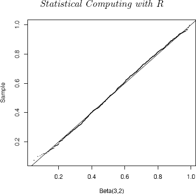
QQ Plot comparing the Beta(3, 2) distribution witha simulated random sample generated by the ratio of gammas method in Example 3.8.
Example 3.9 (Logarithmic distribution, version 2)
This example provides another, more efficient generator for the logarithmic distribution (see Example 3.6). If U, V are independent Uniform(0,1) random variables, then
X=⌊1+log(V)log(1−(1−θ)U)⌋ (3.3)
has the Logarithmic(θ) distribution ([69, pp. 546-8], [159]). This transformation provides a simple and efficient generator for the logarithmic distribution.
Below is a comparison of the Logarithmic(0.5) distribution with a sample generated using transformation (3.3). The empirical probabilities p.hat are within two standard errors of the theoretical probabilities p.
n <- 1000
theta <- 0.5
u <- runif(n) #generate logarithmic sample
v <- runif(n)
x <- floor(1 + log(v) / log(1 - (1 - theta)^u))
k <- 1:max(x) #calc. logarithmic probs.
p <- -1 / log(1 - theta) * theta^k / k
se <- sqrt(p*(1-p)/n)
p.hat <- tabulate(x)/n
> print(round(rbind(p.hat, p, se), 3))
[,1] [,2] [,3] [,4] [,5] [,6] [,7]
p.hat 0.740 0.171 0.052 0.018 0.010 0.006 0.003
p 0.721 0.180 0.060 0.023 0.009 0.004 0.002
se 0.014 0.012 0.008 0.005 0.003 0.002 0.001
The following function is a simple replacement for rlogarithmic in Example 3.6 on page 54.
rlogarithmic <- function(n, theta) {
stopifnot(all(theta > 0 & theta < 1))
th <- rep(theta, length=n)
u <- runif(n)
v <- runif(n)
x <- floor(1 + log(v) / log(1 - (1 - th)^u))
return(x)
}
R note 3.3 The & operator performs an elementwise AND comparison. The && operator evaluates from left to right until a logical result is obtained. For example
x <- 1:5
> 1 < x & x < 5
[1] FALSE TRUE TRUE TRUE FALSE
> 1 < x && x < 5
[1] FALSE
> any(1 < x& x < 5)
[1] TRUE
> any(1 < x && x < 5)
[1] FALSE
> any(1 < x) && any(x < 5)
[1] TRUE
> all(1 < x) && all(x < 5)
[1] FALSE
Similarly, | performs elementwise an OR comparison and || evaluates from left to right.
R note 3.4 The tabulate function bins positive integers, so it can be used on the logarithmic sample. For other types of data, recode the data to positive integers or use Table. If the data are not positive integers, tabulate will truncate real numbers and ignore without warning integers less than 1.
3.5 Sums and Mixtures
Sums and mixtures of random variables are special types of transformations. In this section we focus on sums of independent random variables (convolutions) and several examples of discrete and continuous mixtures.
Convolutions
Let X1, ... , Xn be independent and identically distributed with distribution Xj ~ X, and let S = X1 + · · · + Xn. The distribution function of the sum S is called the n-fold convolution of X and denoted F*(n)x.. It is straightforward to simulate a convolution by directly generating X1, ... , Xn and computing the sum.
Several distributions are related by convolution. If ν > 0 is an integer, the chisquare distribution with ν degrees of freedom is the convolution of ν iid squared standard normal variables. The negative binomial distribution NegBin(r, p) is the convolution of r iid Geom(p) random variables. The convolution of r independent Exp(λ) random variables has the Gamma(r, λ) distribution. See Bean [23] for an introductory level presentation of these and many other interesting relationships between families of distributions.
In R it is of course easier to use the functions rchisq, rgeom and rnbinom to generate chisquare, geometric and negative binomial random samples. The following example is presented to illustrate a general method that can be applied whenever distributions are related by convolutions.
Example 3.10 (Chisquare)
This example generates a chisquare x2(ν) random variable as the convolution of ν squared normals. If Z1, ... , Zν are iid N(0,1) random variables, then V=Z21+ ... +Z2ν has the x2(ν) distribution. Steps to generate a random sample of size n from χ2(ν) are as follows.
- Fill an n × ν matrix with nν random N(0,1) variates.
- Square each entry in the matrix (1).
- Compute the row sums of the squared normals. Each row sum is one random observation from the χ2(ν) distribution.
- Deliver the vector of row sums.
An example with n = 1000 and ν = 2 is shown below.
n <- 1000
nu <- 2
X <- matrix(rnorm(n*nu), n, nu)^2 #matrix of sq. normals
#sum the squared normals across each row: method 1
y <- rowSums(X)
#method 2
y <- apply(X, MARGIN=1, FUN=sum) #a vector length n
> mean(y)
[1] 2.027334
> mean(y^2)
[1] 7.835872
A χ2(ν) random variable has mean ν and variance 2ν. Our sample statistics below agree very closely with the theoretical moments E[Y] = ν = 2 and E[Y2] = 2ν + ν2 = 8. Here the standard errors of the sample moments are 0.063 and 0.089 respectively.
R note 3.5 This example introduces the apply function. The apply function applies a function to the margins of an array. To sum across the rows of matrix X, the function (FUN=sum) is applied to the rows (MARGIN=1). Notice that a loop is not used to compute the row sums. In general for efficient programming in R, avoid unnecessary loops. (For row and column sums it is easier to use rowSums and colSums.)
Mixtures
A random variable X is a discrete mixture if the distribution of X is a weighted sum Fx(x)=∑θiFXi(x) for some sequence of random variables X1, X2,... and θi > 0 such that ∑iθi=1. The constants θi are called the mixing weights or mixing probabilities. Although the notation is similar for sums and mixtures, the distributions represented are different.
A random variable X is a continuous mixture if the distribution of X is FX(x)=∫∞−∞FX|Y=y(x)fY(y) dy for a family X|Y=y indexed by the real numbers y and weighting function fY such that ∫∞−∞fY(y) dy=1
Compare the methods for simulation of a convolution and a mixture of normal variables. Suppose X1 ~ N(0,1) and X2 ~ N(3,1) are independent. The notation S = X1 + X2 denotes the convolution of X1 and X2. The distribution of S is normal with mean μ1 + μ2 = 3 and variance σ21+σ22=2.
To simulate the convolution:
- Generate x1 — N(0, 1).
- Generate x2 — N(3, 1).
- Deliver s = x1 + x2.
We can also define a 50% normal mixture X, denoted FX(x)=0.5Fx1(x)+0.5Fx2(x). Unlike the convolution above, the distribution of the mixture X is distinctly non-normal; it is bimodal.
To simulate the mixture:
1. Generate an integer k ∈ {1, 2}, where P(1) = P(2) = 0.5.
2. If k = 1 deliver random x from N(0, 1);
if k = 2 deliver random x from N(3, 1).
In the following example we will compare simulated distributions of a convolution and a mixture of gamma random variables.
Example 3.11 (Convolutions and mixtures)
Let X1 ~ Gamma(2, 2) and X2 ~ Gamma(2, 4) be independent. Compare the histograms of the samples generated by the convolution S = X1 +X2 and the mixture FX = 0.5FX1 + 0.5FX2.
n <- 1000
x1 <- rgamma(n, 2, 2)
x2 <- rgamma(n, 2, 4)
s <- x1 + x2 #the convolution
u <- runif(n)
k <- as.integer(u > 0.5) #vector of 0’s and 1’s
x <- k * x1 + (1-k) * x2 #the mixture
par(mfcol=c(1,2)) #two graphs per page
hist(s, prob=TRUE)
hist(x, prob=TRUE)
par(mfcol=c(1,1)) #restore display
The histograms shown in Figure 3.3, of the convolution S and mixture X, are clearly different.
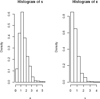
Histogram of a simulated convolution of Gamma(2, 2) and Gamma(2, 4) random variables (left), and a 50% mixture of the same variables(right), from Example 3.11.
R note 3.6 The par function can be used to set (or query) certain graphical parameters. A list of all graphical parameters is returned by par(). The command par(mfcol=c(n,m)) configures the graphical device to display nm graphs per screen, in n rows and m columns.
The method of generating the mixture in this example is simple for a mixture of two distributions, but not for arbitrary mixtures. The next example illustrates how to generate a mixture of several distributions with arbitrary mixing probabilities.
Example 3.12 (Mixture of several gamma distributions)
This example is similar to the previous one, but there are several components to the mixture and the mixing weights are not uniform. The mixture is
FX=5∑i=1θjFXj,
where Xj ~ Gamma(r = 3, λj = 1/j) are independent and the mixing probabilities are θj = j/15, j = 1,..., 5.
To simulate one random variate from the mixture FX:
- Generate an integer k ∈ {1, 2, 3, 4, 5}, where P(k) = θk, k = 1, ..., 5.
- Deliver a random Gamma(r, λk) variate.
To generate a sample size n, steps (1) and (2) are repeated n times. Notice that the algorithm stated above suggests using a for loop, but for loops are really inefficient in R. The algorithm can be translated into a vectorized approach.
- Generate a random sample k1, ... , kn of integers in a vector k, where P(k) = θk, k = 1, ... , 5. Then k[i] indicates which of the five gamma distributions will be sampled to get the i element of the sample (use sample).
- Set rate equal to the length n vector λ = (λk).
- Generate a gamma sample size n, with shape parameter r and rate vector rate (use rgamma).
Then an efficient way to implement this in R is shown by the following example.
n <- 5000
k <- sample(1:5, size=n, replace=TRUE, prob=(1:5)/15)
rate <- 1/k
x <- rgamma(n, shape=3, rate=rate)
#plot the density of the mixture
#with the densities of the components
plot(density(x), xlim=c(0,40), ylim=c(0,.3),
lwd=3, xlab="x", main="”)
for (i in 1:5)
lines(density(rgamma(n, 3, 1/i)))
The plot in Figure 3.4 shows the density of each Xj and the density of the mixture (thick line). The density curves in Figure 3.4 are actually density estimates, which will be discussed in Chapter 10.
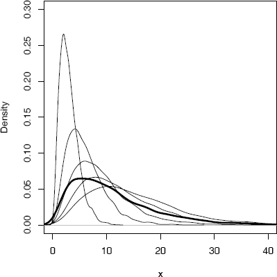
Density estimates from Example 3.12: A mixture (thick line) of several gamma densities (thin lines).
Example 3.13 (Mixture of several gamma distributions)
Let
FX=5∑i=1θjFXj
where Xj ~ Gamma(3, λj) are independent, with rates λ = (1, 1.5,2,2.5,3), and mixing probabilities θ = (0.1, 0.2, 0.2, 0.3, 0.2).
This example is similar to the previous one. Sample from 1:5 with probability weights θ to get a vector length n. The ith position in this vector indicates which of the five gamma distributions is sampled to get the ith element of the sample. This vector is used to select the correct rate parameter from the vector λ.
n <- 5000
p <- c(.1,.2,.2,.3,.2)
lambda <- c(1,1.5,2,2.5,3)
k <- sample(1:5, size=n, replace=TRUE, prob=p)
rate <- lambda[k]
x <- rgamma(n, shape=3, rate=rate)
Note that lambda[k] is a vector the same length as k, containing the elements of lambda indexed by the vector k. In mathematical notation, lambda[k] is equal (λk1,λk2,...,λkn).
Compare the first few entries of k and the corresponding values of rate with λ.
> k[1:8]
[1] 5 1 4 2 1 3 2 3
> rate[1:8]
[1] 3.0 1.0 2.5 1.5 1.0 2.0 1.5 2.0
Example 3.14 (Plot density of mixture)
Plot the densities (not density estimates) of the gamma distributions and the mixture in Example 3.13. (This example is a programming exercise that involves vectors of parameters and repeated use of the apply function.)
The density of the mixture is
f(x)=5∑j=1θjfj(x), x>0, (3.4)
where fj is the Gamma(3, λj) density. To produce the plot, we need a function to compute the density f(x) of the mixture.
f <- function(x, lambda, theta) {
#density of the mixture at the point x
sum(dgamma(x, 3, lambda) * theta)
}
The function f computes the density of the mixture (3.4) for a single value of x. If x has length 1, dgamma(x, 3, lambda) is a vector the same length as lambda; in this case (f1(x),..., f5(x)). Then dgamma(x, 3, lambda)*theta is the vector (θ1f1(x), ... , θ5f5(x)). The sum of this vector is the density of the mixture (3.3) evaluated at the point x.
x <- seq(0, 8, length=200)
dim(x) <- length(x) #need for apply
#compute density of the mixture f(x) along x
y <- apply(x, 1, f, lambda=lambda, theta=p)
The density of the mixture is computed by function f applied to the vector x. The function f takes several arguments, so the additional arguments lambda=lambda, theta=prob are supplied after the name of the function, f.
A plot of the five densities with the mixture is shown in Figure 3.5. The code to produce the plot is listed below. The densities fk can be computed by the dgamma function. A sequence of points x is defined and each of the densities are computed along x.
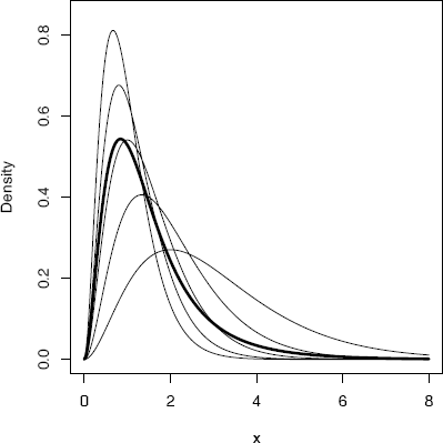
Densities from Example 3.14: A mixture (thick line) of several gamma densities (thin lines).
#plot the density of the mixture
plot(x, y, type="l", ylim=c(0,.85), lwd=3, ylab="Density”)
for (j in 1:5) {
#add the j-th gamma density to the plot
y <- apply(x, 1, dgamma, shape=3, rate=lambda[j])
lines(x, y)
}
R note 3.7 The apply function requires a dimension attribute for x. Since x is a vector, it does not have a dimension attribute by default. The dimension of x is assigned by dim(x) <- length(x). Alternately, x <- as.matrix(x) converts x to a matrix (a column vector), which has a dimension attribute.
Example 3.15 (Poisson-Gamma mixture)
This is an example of a continuous mixture. The negative binomial distribution is a mixture of Poisson(Λ) distributions, where Λ has a gamma distribution. Specifically, if (X|Λ = λ) ~ Poisson(λ) and Λ ~ Gamma(r, β), then X has the negative binomial distribution with parameters r and p = β/(1 + β) (see e.g. [23]). This example illustrates a method of sampling from a Poisson-Gamma mixture and compares the sample with the negative binomial distribution.
#generate a Poisson-Gamma mixture
n <- 1000
r <- 4
beta <- 3
lambda <- rgamma(n, r, beta) #lambda is random
#now supply the sample of lambda’s as the Poisson mean
x <- rpois(n, lambda) #the mixture
#compare with negative binomial
mix <- tabulate(x+1) / n
negbin <- round(dnbinom(0:max(x), r, beta/(1+beta)), 3)
se <- sqrt(negbin * (1 - negbin) / n)
The empirical distribution (first line below) of the mixture agrees very closely with the pmf of NegBin(4, 3/4) (second line).
> round(rbind(mix, negbin, se), 3)
[,1] [,2] [,3] [,4] [,5] [,6] [,7] [,8] [,9]
mix 0.334 0.305 0.201 0.091 0.042 0.018 0.005 0.003 0.001
negbin 0.316 0.316 0.198 0.099 0.043 0.017 0.006 0.002 0.001
se 0.015 0.015 0.013 0.009 0.006 0.004 0.002 0.001 0.001
3.6 Multivariate Distributions
Generators for the multivariate normal distribution, multivariate normal mixtures, Wishart distribution, and uniform distribution on the sphere in ℝd are presented in this section.
3.6.1 Multivariate Normal Distribution
A random vector X = (X1, ... , Xd) has a d-dimensional mutivariate normal (MVN) distribution denoted Nd(µ, Σ) if the density of X is
f(x)=1(2π)d2|Σ|12exp{−(12)(x−μ)}, x∈ℝd, (3.5)
where µ = (µ1, ... , µd)T is the mean vector and Σ is a d × d symmetric positive
definite matrix
∑=[σ11σ12⋯σ1dσ21σ22⋯σ2d⋮⋮⋮σd1σd2⋯σdd]
with entries σij = Cov(Xi, Xj). Here Σ−1 is the inverse of Σ, and |Σ| is the determinant of Σ. The bivariate normal distribution is the special case N2(µ, Σ).
A random Nd(µ, Σ) variate can be generated in two steps. First generate Z = (Z1, ... , Zd), where Z1, ... , Zd are iid standard normal variates. Then transform the random vector Z so that it has the desired mean vector µ and covariance structure Σ. The transformation requires factoring the covariance matrix Σ.
Recall that if Z ~ Nd(µ, Σ), then the linear transformation CZ + b is multivariate normal with mean Cµ+b and covariance CΣCT . If Z is Nd(0, Id), then
CZ+b~Nd(b,CCT).
Suppose that Σ can be factored so that Σ = CCT for some matrix C. Then
CZ+μ~Nd(μ,∑),
and CZ+µ is the required transformation.
The required factorization of Σ can be obtained by the spectral decomposition method (eigenvector decomposition), Choleski factorization, or singular value decomposition (svd). The corresponding R functions are eigen, chol, and svd.
Usually, one does not apply a linear transformation to the random vectors of a sample one at a time. Typically, one applies the transformation to a data matrix and transforms the entire sample. Suppose that Z = (Zij) is an n × d matrix where Zij are iid N(0,1). Then the rows of Z are n random observations from the d-dimensional standard MVN distribution. The required transformation applied to the data matrix is
X=ZQ+JμT,(3.6)
where QT Q = Σ and J is a column vector of ones. The rows of X are n random observations from the d-dimensional MVN distribution with mean vector μ and covariance matrix Σ.
Method for generating multivariate normal samples
To generate a random sample of size n from the Nd(µ, Σ) distribution:
- Generate an n × d matrix Z containing nd random N(0,1) variates (n random vectors in ℝd).
- Compute a factorization Σ = QT Q.
- Apply the transformation X = ZQ + JµT.
- Deliver the n × d matrix X.
Each row of X is a random variate from the Nd(µ, Σ) distribution.
The X = ZQ + JµT transformation can be coded in R as follows. Recall that the matrix multiplication operator is %*%.
Z <- matrix(rnorm(n*d), nrow = n, ncol = d)
X <- Z %*% Q + matrix(mu, n, d, byrow = TRUE)
The matrix product JµT is equal to matrix(mu, n, d, byrow = TRUE). This saves a matrix multiplication. The argument byrow = TRUE is necessary here; the default is byrow = FALSE. The matrix is filled row by row with the entries of the mean vector mu.
In this section each method of generating MVN random samples is illustrated with examples. Also note that there are functions provided in R packages for generating multivariate normal samples. See the mvrnorm function in the MASS package [278], and rmvnorm in the mvtnorm package [115]. In all of the examples below, the rnorm function is used to generate standard normal random variates.
Spectral decomposition method for generating Nd(µ, ∑) samples
The square root of the covariance is Σ1/2 = P∧1/2P-1, where Λ is the diagonal matrix with the eigenvalues of E along the diagonal and P is the matrix whose columns are the eigenvectors of Σ corresponding to the eigenvalues in ∧. This method can also be called the eigen-decomposition method. In the eigen-decomposition we have P−1 = PT and therefore Σ1/2 = P∧1/2PT. The matrix Q = Σ1/2 is a factorization of E such that QT Q = Σ.
Example 3.16 (Spectral decomposition method)
This example provides a function rmvn.eigen to generate a multivariate normal random sample. It is applied to generate a bivariate normal sample with zero mean vector and
∑=[1.00.90.91.0]
# mean and covariance parameters
mu <- c(0, 0)
Sigma <- matrix(c(1, .9, .9, 1), nrow = 2, ncol = 2)
The eigen function returns the eigenvalues and eigenvectors of a matrix.
rmvn.eigen <-
function(n, mu, Sigma) {
# generate n random vectors from MVN(mu, Sigma)
# dimension is inferred from mu and Sigma
d <- length(mu)
ev <- eigen(Sigma, symmetric = TRUE)
lambda <- ev$values
V <- ev$vectors
R <- V %*% diag(sqrt(lambda)) %*% t(V)
Z <- matrix(rnorm(n*d), nrow = n, ncol = d)
X <- Z %*% R + matrix(mu, n, d, byrow = TRUE)
X
}
Print summary statistics and display a scatterplot as a check on the results of the simulation.
# generate the sample
X <- rmvn.eigen(1000, mu, Sigma)
plot(X, xlab = “x”, ylab = “y”, pch = 20)
> print(colMeans(X))
[1] -0.001628189 0.023474775
> print(cor(X))
[,1] [,2]
[1,] 1.0000000 0.8931007
[2,] 0.8931007 1.0000000
Output from Example 3.16 shows the sample mean vector is (−0.002, 0.023) and sample correlation is 0.893, which agree closely with the specified parameters. The scatter plot of the sample data shown in Figure 3.6 exhibits the elliptical symmetry of multivariate normal distributions.
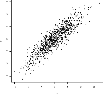
Scatterplot of a random bivariate normal sample with mean vector zero, variances σ21=σ22=1 and correlation ρ = 0.9, from Example 3.16.
SVD Method of generating Nd(µ, Σ) samples
The singular value decomposition (svd) generalizes the idea of eigenvectors to rectangular matrices. The svd of a matrix X is X = UDVT , where D is a vector containing the singular values of X, U is a matrix whose columns contain the left singular vectors of X, and V is a matrix whose columns contain the right singular vectors of X. The matrix X in this case is the population covariance matrix Σ, and UVT = I. The svd of a symmetric positive definite matrix ∑ gives U = V = P and Σ1/2 = UD1/2VT. Thus the svd method for this application is equivalent to the spectral decomposition method, but is less efficient because the svd method does not take advantage of the fact that the matrix ∑ is square symmetric.
Example 3.17 (SVD method)
This example provides a function rmvn.svd to generate a multivariate normal sample, using the svd method to factor ∑.
rmvn.svd <-
function(n, mu, Sigma) {
# generate n random vectors from MVN(mu, Sigma)
# dimension is inferred from mu and Sigma
d <- length(mu)
S <- svd(Sigma)
R <- S$u %*% diag(sqrt(S$d)) %*% t(S$v) #sq. root Sigma
Z <- matrix(rnorm(n*d), nrow=n, ncol=d)
X <- Z %*% R + matrix(mu, n, d, byrow=TRUE)
X
}
This function is applied in Example 3.19 on page 76.
Choleski factorization method of generating Nd(µ, Σ) samples
The Choleski factorization of a real symmetric positive-definite matrix is X = QT Q, where Q is an upper triangular matrix. The Choleski factorization is implemented in the R function chol. The basic syntax is chol(X) and the return value is an upper triangular matrix R such that RT R = X.
Example 3.18 (Choleski factorization method)
The Choleski factorization method is applied to generate 200 random observations from a four-dimensional multivariate normal distribution.
rmvn.Choleski <-
function(n, mu, Sigma) {
# generate n random vectors from MVN(mu, Sigma)
# dimension is inferred from mu and Sigma
d <- length(mu)
Q <- chol(Sigma) # Choleski factorization of Sigma
Z <- matrix(rnorm(n*d), nrow=n, ncol=d)
X <- Z %*% Q + matrix(mu, n, d, byrow=TRUE)
X
}
In this example, we will generate the samples according to the same mean and covariance structure as the four-dimensional iris virginica data.
y <- subset(x=iris, Species=="virginica”)[, 1:4]
mu <- colMeans(y)
Sigma <- cov(y)
> mu
Sepal.Length Sepal.Width Petal.Length Petal.Width
6.588 2.974 5.552 2.026
> Sigma
Sepal.Length Sepal.Width Petal.Length Petal.Width
Sepal.Length 0.40434286 0.09376327 0.30328980 0.04909388
Sepal.Width 0.09376327 0.10400408 0.07137959 0.04762857
Petal.Length 0.30328980 0.07137959 0.30458776 0.04882449
Petal.Width 0.04909388 0.04762857 0.04882449 0.07543265
#now generate MVN data with this mean and covariance
X <- rmvn.Choleski(200, mu, Sigma)
pairs(X)
The pairs plot of the data in Figure 3.7 gives a 2-D view of the bivariate distribution of each pair of marginal distributions. The joint distribution of each pair of marginal distributions is theoretically bivariate normal. The plot can be compared with Figure 4.1, which displays the iris virginica data. (The iris virginica data are not multivariate normal, but means and correlation for each pair of variables should be similar to the simulated data.)
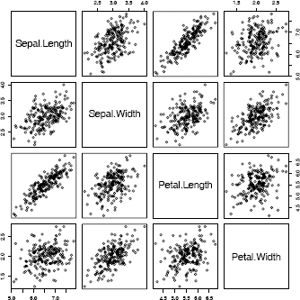
Pairs plot of the bivariate marginal distributions of a simulated multivariate normal random sample in Example 3.18. The parameters match the mean and covariance of the iris virginica data.
Remark 3.3 To standardize a multivariate normal sample, we invert the procedure above, substituting the sample mean vector and sample covariance matrix if the parameters are unknown. The transformed d-dimensional sample then has zero mean vector and covariance Id. This is not the same as scaling the columns of the data matrix.
Comparing Performance of Generators
We have discussed several methods for generating random samples from specified probability distributions. When several methods are available, which method is preferred? One consideration may be the computational time required (the time complexity). Another important consideration, if the purpose of the simulation is to estimate one or more parameters, is the variance of the estimator. The latter topic is considered in Chapter 5. To compare the empirical performance with respect to computing time, we can time each procedure.
R provides the system.time function, which times the evaluation of its argument. This function can be used as a rough benchmark to compare the performance of different algorithms. In the next example, the system.time function is used to compare the CPU time required for several different methods of generating multivariate normal samples.
Example 3.19 (Comparing performance of MVN generators)
This example generates multivariate normal samples in a higher dimension (d = 30) and compares the timing of each of the methods presented in Section 3.6.1 and two generators available in R packages. This example uses a function rmvnorm in the package mvtnorm [115]. This package is not part of the standard R distribution but can be installed from CRAN. The MASS package [278] is one of the recommended packages included with the R distribution.
library(MASS)
library(mvtnorm)
n <- 100 #sample size
d <- 30 #dimension
N <- 2000 #iterations
mu <- numeric(d)
set.seed(100)
system.time(for (i in 1:N)
rmvn.eigen(n, mu, cov(matrix(rnorm(n*d), n, d))))
set.seed(100)
system.time(for (i in 1:N)
rmvn.svd(n, mu, cov(matrix(rnorm(n*d), n, d))))
set.seed(100)
system.time(for (i in 1:N)
rmvn.Choleski(n, mu, cov(matrix(rnorm(n*d), n, d))))
set.seed(100)
system.time(for (i in 1:N)
mvrnorm(n, mu, cov(matrix(rnorm(n*d), n, d))))
set.seed(100)
system.time(for (i in 1:N)
rmvnorm(n, mu, cov(matrix(rnorm(n*d), n, d))))
set.seed(100)
system.time(for (i in 1:N)
cov(matrix(rnorm(n*d), n, d)))
Most of the work involved in generating a multivariate normal sample is the factorization of the covariance matrix. The covariances used for this example are actually the sample covariances of standard multivariate normal samples. Thus, the randomly generated ∑ varies with each iteration, but ∑ is close to an identity matrix. In order to time each method on the same covariance matrices, the random number seed is restored before each run. The last run simply generates the covariances, for comparison with the total time.
The results below (summarized from the console output) suggest that there are differences in performance among these five methods when the covariance matrix is close to identity. The Choleski method is somewhat faster, while rmvn.eigen and mvrnorm (MASS) [278] appear to perform about equally well. The similar performance of rmvn.eigen and mvrnorm is not surprising, because according to the documentation for mvrnorm, the method of matrix decomposition is the eigendecomposition. Documentation for mvrnorm states that “although a Choleski decomposition might be faster, the eigendecomposition is stabler.”
Timings of MVN generators
user system elapsed
rmvn.eigen 7.36 0.00 7.37
rmvn.svd 9.93 0.00 9.94
rmvn.choleski 5.32 0.00 5.35
mvrnorm 7.95 0.00 7.96
rmvnorm 11.91 0.00 11.93
generate Sigma 2.78 0.00 2.78
The system.time function was also used to compare the methods in Examples 3.22 and 3.23. The code (not shown) is similar to the examples above.
3.6.2 Mixtures of Multivariate Normals
A multivariate normal mixture is denoted
pNd(μ1,∑1)+(1−p)Nd(μ2,Σ2) (3.7)
where the sampled population is Nd(µ1, Σ1) with probability p, and Nd(µ2, Σ2) with probability 1 − p. As the mixing parameter p and other parameters are varied, the multivariate normal mixtures have a wide variety of types of departures from normality. For example, a 50% normal location mixture is symmetric with light tails, and a 90% normal location mixture is skewed with heavy tails. A normal location mixture with p=1−12(1−√33)≐0.7887, provides an example of a skewed distribution with normal kurtosis [140]. Parameters can be varied to generate a wide variety of distributional shapes. Johnson [154] gives many examples for the bivariate normal mixtures. Many commonly applied statistical procedures do not perform well under this type of departure from normality, so normal mixtures are often chosen to compare the properties of competing robust methods of analysis.
If X has the distribution (3.7) then a random observation from the distribution of X can be generated as follows.
To generate a random sample from pNd(µ1, Σ1) + (1 − p)Nd(µ2, Σ2)
- Generate U ~ Uniform(0,1).
- If U ≤ p generate X from Nd(µ1, Σ1);
otherwise generate X from Nd(µ2, Σ2).
The following procedure is equivalent.
- Generate N ~ Bernoulli(p).
- If N = 1 generate X from Nd(µ1, Σ1);
otherwise generate X from Nd(µ2, Σ2).
Example 3.20 (Multivariate normal mixture)
Write a function to generate a multivariate normal mixture with two components. The components of a location mixture differ in location only. Use the mvrnorm(MASS) function [278] to generate the multivariate normal observations.
First we write this generator in an inefficient loop to clearly illustrate the steps outlined above. (We will eliminate the loop later.)
library(MASS) #for mvrnorm
#ineffecient version loc.mix.0 with loops
loc.mix.0 <- function(n, p, mu1, mu2, Sigma) {
#generate sample from BVN location mixture
X <- matrix(0, n, 2)
for (i in 1:n) {
k <- rbinom(1, size = 1, prob = p)
if (k)
X[i,]<- mvrnorm(1, mu = mu1, Sigma) else
X[i,]<- mvrnorm(1, mu = mu2, Sigma)
}
return(X)
}
Although the code above will generate the required mixture, the loop is rather inefficient. Generate n1, the number of observations realized from the first component, from Binomial(n,p). Generate n1 variates from component 1 and n2 = n − n1 from component 2 of the mixture. Generate a random permutation of the indices 1:n to indicate the order in which the sample observations appear in the data matrix. See Appendix B.1 for details about permutations of rows of a matrix.
#more efficient version
loc.mix <- function(n, p, mu1, mu2, Sigma) {
#generate sample from BVN location mixture
n1 <- rbinom(1, size = n, prob = p)
n2 <- n - n1
x1 <- mvrnorm(n1, mu = mu1, Sigma)
x2 <- mvrnorm(n2, mu = mu2, Sigma)
X <- rbind(x1, x2) #combine the samples
return(X[sample(1:n),]) #mix them
}
To illustrate the normal mixture generator, we apply loc.mix to generate a random sample of n = 1000 observations from a 50% 4-dimensional normal location mixture with µ1 = (0, 0, 0, 0) and µ2 = (2, 3, 4, 5) and covariance I4.
x <- loc.mix(1000, .5, rep(0, 4), 2:5, Sigma = diag(4))
r <- range(x) * 1.2
par(mfrow = c(2, 2))
for (i in 1:4)
hist(x[, i], xlim = r, ylim = c(0, .3), freq = FALSE,
main = "", breaks = seq(-5, 10, .5))
par(mfrow = c(1, 1))
It is difficult to visualize data in ℝ4 , so we display only the histograms of the marginal distributions in Figure 3.8. All of theone dimensional marginal distributions are univariate normal location mixtures. Methods for visualization of multivariate data are covered in Chapter 4. Also, an interesting view ofa bivariate normal mixture with three components is shown in Figure 10.13 on page 313.
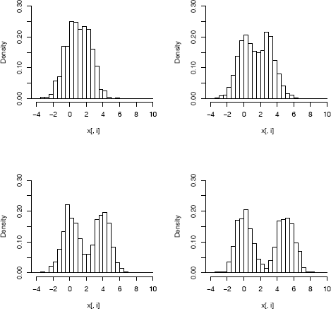
Histograms of the marginal distributions of multivariate normal location mixture data generated in Example 3.20.
3.6.3 Wishart Distribution
Suppose M = XTX, where X is an n × d data matrix of a random sample from a Nd(µ, Σ) distribution. Then M has a Wishart distribution with scale matrix E and n degrees of freedom, denoted M ~ Wd(Σ, n) (see e.g. [8, 188]). Note that when d = 1, the elements of X are a univariate random sample from N(µ, σ2) so w1(σ2,n)D=σ2χ2(n).
An obvious, but inefficient approach to generating random variates from a Wishart distribution, is to generate multivariate normal random samples and compute the matrix product XTX. This method is computationally expensive because nd random normal variates must be generated to determine the d(d + 1)/2 distinct entries in M.
A more efficient method based on Bartlett’s decomposition [21] is summarized by Johnson [154, p. 204] as follows. Let T = (Tij) be a lower triangular d × d random matrix with independent entries satisfying
- Tijiid~N(0,1),i>j.
- Tij~√χ2(n−i+1),i=1,...,d
Then the matrix A = TTT has a Wd(Id, n) distribution. To generate Wd(Σ, n) random variates, obtain the Choleski factorization Σ = LLT, where L is lower triangular. Then LALT ~ Wd(Σ, n) [21, 133, 207]. Implementation is left as an exercise.
3.6.4 Uniform Distribution on the d-Sphere
The d-sphere is the set of all points x∈ℝd such that ||x||=(xTx)12=1. Random vectors uniformly distributed on the d-sphere have equally likely directions. A method of generating this distribution uses a property of the multivariate normal distribution (see e.g. [94, 154]). If X1, ... , Xd are iid N(0,1), then U = (U1, ... , Ud) is uniformly distributed on the unit sphere in ℝd, where
Uj=Xj(X21+...+X2d), j=1,...,d (3.8)
Algorithm to generate uniform variates on the d-Sphere
- For each variate ui, i = 1, ... , n repeat
- Generate a random sample xi1, ... , xid from N(0,1).
- Compute the Euclidean norm .
- Set
- Deliver
To implement these steps efficiently in R for a sample size n,
- Generate nd univariate normals in n x d matrix M. The ith row of M corresponds to to the ith random vector ui.
- Compute the denominator of (3.8) for each row, storing the n norms in vector L.
- Divide each number M[i,j] by the norm L[i], to get the matrix U, where U[i,] = ui = (ui1,...,uid).
- Deliver matrix U containing n random observations in rows.
Example 3.21 (Generating variates on a sphere)
This example provides a function to generate random variates uniformly distributed on the unit d-sphere.
runif.sphere <- function(n, d) {
# return a random sample uniformly distributed
# on the unit sphere in R ^d
M <- matrix(rnorm(n*d), nrow = n, ncol = d)
L <- apply(M, MARGIN = 1,
FUN = function(x){sqrt(sum(x*x))})
D <- diag(1 / L)
U <- D %*% M
U
}
The function runif.sphere is used to generate a sample of 200 points uniformly distributed on the circle.
#generate a sample in d=2 and plot
X <- runif.sphere(200, 2)
par(pty = "s")
plot(X, xlab = bquote(x[1]), ylab = bquote(x[2]))
par(pty = "m")
The circle of points is shown in Figure 3.9.
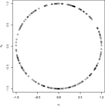
A random sample of 200 points from the bivariate distribution (X1,X2) that is uniformly distributed on the unit circle in Example 3.21.
R note 3.8 The apply function in runif.sphere returns a vector containing then norms ||x1||, ||x2||, ... , ||xn|| of the sample vectors in matrix M.
R note 3.9 The command par(pty = "s") sets the square plot type so the circle is round rather than elliptical; par(pty = "m") restores the type to maximal plotting region. See the help topic ?par for other plot parameters.
Uniformly distributed points on a hyperellipsoid can be generated by applying a suitable linear transformation to a Uniform sample on the d-sphere. Fishman [94, 3.28] gives an algorithm for generating points in and on a simplex.
3.7 Stochastic Processes
A stochastic process is a collection {X(t) : t ∈ T} of random variables indexed by the set T, which usually represents time. The index set T, could be discrete or continuous. The set of possible values X(t) can take is the state space, which also can be discrete or continuous. Ross [234] is an excellent introduction to stochastic processes, and includes a chapter on simulation.
A counting process records the number of events or arrivals that occur by time t. A counting process has independent increments if the number of arrivals in disjoint time intervals are independent. A counting process has stationary increments if the number of events occurring in an interval depends only on the length of the interval. An example of a counting process is a Poisson process.
To study a counting process through simulation, we can generate a realization of the process that records events for a finite period of time. The set of times of consecutive arrivals records the outcome and determines the state X(t) at any time t. In a simulation, the sequence of arrival times must be finite. One method of simulation for a counting process is to choose a sufficiently long time interval and generate the arrival times or the interarrival times in this interval.
Poisson Processes
A homogeneous Poisson process {N(t), t ≥ 0} with rate λ is a counting process, with independent increments, such that N(0) = 0 and
Thus, a homogeneous Poisson process has stationary increments and the number of events N(t) in [0, t] has the Poisson(λt) distribution. If T1 is the time until the first arrival,
,
so T1 is exponentially distributed with rate λ. The interarrival times T1, T2,... are the times between successive arrivals. The interarrival times are iid exponentials with rate λ, which follows from (3.9) and the memoryless property of the exponential distribution.
One method of simulating a Poisson process is to generate the interarrival times. Then the time of the nth arrival is the sum Sn = T1 + · · · + Tn (the waiting time until nth arrival). A sequence of interarrival times or sequence of arrival times are a realization of the process. Thus, a realization is an infinite sequence, rather than a single number. In a simulation, the finite sequence of interarrival times arrival times or arrival times are a simulated realization of the process on the interval [0, SN).
Another method of simulating a Poisson process is to use the fact that the conditional distribution of the (unordered) arrival times given N(t) = n is the same as that of a random sample of size n from a Uniform(0, t) distribution.
The state of the process at a given time t is equal to the number of arrivals in [0, t], which is the number min(k : Sk > t)−1. That is, N(t) = n−1, where Sn is the smallest arrival time exceeding t.
Algorithm for simulating a homogeneous Poisson process on an interval [0, t0] by generating interarrival times.
- Set S1 = 0.
- For j = 1, 2,... while Sj ≤ t0:
- Generate Tj — Exp(λ).
- Set Sj = T1 + ··· + Tj.
- N(t0) = minj(Sj > t0) — 1.
It is inefficient to implement this algorithm in R using a for loop. It should be translated into vectorized operations, as shown in the next example.
Example 3.22 (Poisson process)
This example illustrates a simple approach to simulation of a Poisson process with rate λ. Suppose we need N(3), the number of arrivals in [0, 3]. Generate iid exponential times Ti with rate λ and find the index n where the cumulative sum Sn = T1 + · · · + Tn first exceeds 3. It follows that the number of arrivals in [0, 3] is n — 1. On average this number is E[N(3)] = 3λ.
lambda <- 2
t0 <- 3
Tn <- rexp(100, lambda) #interarrival times
Sn <- cumsum(Tn) #arrival times
n <- min(which(Sn > t0)) #arrivals+1 in [0, t0]
Results from two runs are shown below.
> n-1
[1] 8
> round(Sn[1:n], 4)
[1] 1.2217 1.3307 1.3479 1.4639 1.9631 2.0971
2.3249 2.3409 3.9814
> n-1
[1] 5
> round(Sn[1:n], 4)
[1] 0.4206 0.8620 1.0055 1.6187 2.6418 3.4739
For this example, the average of simulated values N(3) = n — 1 for a large number of runs should be close to E[N(3)] = 3λ = 6.
An alternate method of generating the arrival times of a Poisson process is based on the fact that given the number of arrivals in an interval (0, t), the conditional distribution of the unordered arrival times are uniformly distributed on (0, t). That is, given that the number of arrivals in (0, t) is n, the arrival times Sl, ... , Sn, are jointly distributed as an ordered random sample of size n from a Uniform(0, t) distribution.
Applying the conditional distribution of the arrival times, it is possible to simulate a Poisson(λ) process on an interval (0, t) by first generating a random observation n from the Poisson( λt) distribution, then generating a random sample of n Uniform(0, t) observations and ordering the uniform sample to obtain the arrival times.
Example 3.23 (Poisson process, cont.)
Returning to Example 3.22, simulate a Poisson(λ) process and find N(3), using the conditional distribution of the arrival times. As a check, we estimate the mean and variance of N(3) from 10000 replications.
lambda <- 2
t0 <- 3
upper <- 100
pp <- numeric(10000)
for (i in 1:10000) {
N <- rpois(1, lambda * upper)
Un <- runif(N, 0, upper) #unordered arrival times
Sn <- sort(Un) #arrival times
n <- min(which(Sn> t0)) #arrivals+1 in [0, t0]
pp[i] <- n - 1 #arrivals in [0, t0]
}
Alternately, the loop can be replaced by replicate, as shown.
pp <- replicate(10000, expr = {
N <- rpois(1, lambda * upper)
Un <- runif(N, 0, upper) #unordered arrival times
Sn <- sort(Un) #arrival times
n <- min(which(Sn > t0)) #arrivals+1 in [0, t0]
n - 1}) #arrivals in [0, t0]
The mean and variance should both be equal to λt = 6 in this example. Here the sample mean and sample variance of the generated values N(3) are indeed very close to 6.
> c(mean(pp), var(pp))
[1] 5.977100 5.819558
Actually, it is possible that none of the generated arrival times exceed the time t0 = 3. In this case, the process needs to be simulated for a longer time than the value in upper. Therefore, in practice, one should choose upper according to the parameters of the process, and do some error checking. For example, if we need N(t0), one approach is to wrap the min(which()) step with try and check that the result of try is an integer using is.integer. See the corresponding help topics for details.
Ross [234] discusses the computational efficiency of the two methods applied in Examples 3.22 and 3.23. Actually, the second method is considerably slower (by a factor of 4 or 5) than the previous method of Example 3.22 when coded in R. The rexp generator is almost as fast as runif, while the sort operation adds O(nlog(n)) time. Some performance improvement might be gained if this algorithm is coded in C and a faster sorting algorithm designed for uniformnumbers is used.
Nonhomogeneous Poisson Processes
A counting process is a Poisson process with intensity function λ(t), t ≥ 0 if N(t) = 0, N(t) has independent increments, and for h > 0,
The Poisson process N(t) is nonhomogeneous if the intensity function λ(t) is not constant. A nonhomogeneous Poisson process has independent increments but does not have stationary increments. The distribution of
is Poisson with mean The function is called the mean value function of the process. Note that m(t) = λ in the case of the homogeneous Poisson process, where the intensity function is a constant.
Every nonhomogeneous Poisson process with a bounded intensity function can be obtained by time sampling a homogeneous Poisson process. Suppose that λ(t) ≤ λ < ∞ for all t ≥ 0. Then sampling a Poisson(λ) process such that an event happening at time t is accepted or counted with probability λ(t)/λ generates the nonhomogeneous process with intensity function λ(t). To see this, let N(t) be the number of accepted events in [0, t]. Then N(t) has the Poisson distribution with mean
To simulate a nonhomogeneous Poisson process on an interval [0, t0], find λ0 < ∞ such that λ(t) < = λ0, 0 ≤ t ≤ t0. Then generate from the homogeneous Poisson(λ0) process the arrival times {Sj}, and accept each arrival with probability λ(Sj)/λ0. The steps to simulate the process on an interval [0, t0) are as follows.
Algorithm for simulating a nonhomogeneous Poisson process on an interval [0, t0] by sampling from a homogeneous Poisson process.
- Set S1 = 0.
- For j = 1, 2,... while Sj ≤ t0:
- Generate Tj — Exp(λ0) and set Sj = T1 + ... + Tj.
- Generate Uj — Uniform(0,1).
- If Uj ≤ λ(Sj)/λ0 accept (count) this arrival and set Ij = 1; otherwise Ij = 0.
- Deliver the arrival times {Sj : Ij = 1}.
Although this algorithm is quite simple, for implementation in R it is more efficient if translated into vectorized operations. This is shown in the next example.
Example 3.24 (Nonhomogeneous Poisson process)
Simulate a realization from a nonhomogeneous Poisson process with intensity function λ(t) = 3cos2(t). Here the intensity function is bounded above by λ = 3, so the jth arrival is accepted if Uj ≤ 3 cos2(Sj)/3 = cos2(Sj).
lambda <- 3
upper <- 100
N <- rpois(1, lambda * upper)
Tn <- rexp(N, lambda)
Sn <- cumsum(Tn)
Un <- runif(N)
keep <- (Un <- cos(Sn)^2) #indicator, as logical vector
Sn[keep]
Now, the values in Sn[keep] are the ordered arrival times of the nonhomogeneous Poisson process.
> round(Sn[keep], 4)
[1] 0.0237 0.5774 0.5841 0.6885 2.3262
2.4403 2.9984 3.4317 3.7588 3.9297
[11] 4.2962 6.2602 6.2862 6.7590 6.8354
7.0150 7.3517 8.3844 9.4499 9.4646 ...
To determine the state of the process at time t = 2π, for example, refer to the entries of Sn indexed by keep.
> sum(Sn[keep] <= 2*pi)
[1] 12
> table(keep)/N keep
keep
FALSE TRUE
0.4969325 0.5030675
Thus N(2π) = 12, and in this example approximately 50% of the arrivals were counted.
Renewal Processes
A renewal process is a generalization of the Poisson process. If {N(t), t ≥ 0} is a counting process, such that the sequence of nonnegative interarrival times T1, T2,... are iid (not necessarily exponential distribution), then {N(t), t ≥ 0} is a renewal process. The function m(t) = E[N(t)] is called the mean value function of the process, which uniquely determines the distribution of the interarrival times.
If the distribution FT(t) of the iid interarrival times is specified, then a renewal process can be simulated by generating the sequence of interarrival times, by a method similar to Example 3.22.
Example 3.25 (Renewal process)
Suppose the interarrival times of a renewal process have the geometric distribution with success probability p. (This example is discussed in [234, Sec. 7.2].) Then the interarrival times are nonnegative integers, and Sj = T1 + · · · + Tj have the negative binomial distribution with size parameter r = j and probability p. The process can be simulated by generating geometric interarrival times and computing the consecutive arrival times by the cumulative sum of interarrival times.
t0 <- 5
Tn <- rgeom(100, prob = .2) #interarrival times
Sn <- cumsum(Tn) #arrival times
n <- min(which(Sn > t0)) #arrivals+1 in [0, t0]
The distribution of N(t0) can be estimated by replicating the simulation above.
Nt0 <- replicate(1000, expr = {
Sn <- cumsum(rgeom(100, prob = .2))
min(which(Sn > t0)) - 1
})
table(Nt0)/1000
Nt0
0 1 2 3 4 5 6 7
0.273 0.316 0.219 0.108 0.053 0.022 0.007 0.002
To estimate the means E[N(t)], vary the time t0.
t0 <- seq(0.1, 30, .1)
mt <- numeric(length(t0))
for (i in 1:length(t0)) {
mt[i] <- mean(replicate(1000,
{
Sn <- cumsum(rgeom(100, prob = .2))
min(which(Sn > t0[i])) - 1
}))
}
plot(t0, mt, type = "l", xlab = "t", ylab = "mean")
Let us compare with the homogeneous Poisson process, where the interarrival times have a constant mean. Here we have p = 0.2 so the average interarrival time is 0.8/0.2 = 4. The Poisson process that has mean interarrival time 4 has Poisson parameter λt = t/4. We added a reference line to the plot corresponding to the Poisson process mean λt = t/4 using abline(0, .25).
The plot is shown in Figure 3.10. It should not be surprising that the mean of the renewal process is very close to λt, because the geometric distribution is the discrete analog of exponential; it has the memoryless property. That is, if X ~ Geometric(p), then for all j, k = 0, 1, 2, ...
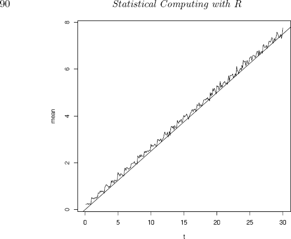
Sequence of sample means of a simulated renewal process in Example 3.25. The reference line corresponds to the mean λt = t/4 of a homogeneous Poisson process.
Symmetric Random Walk
Let X1, X2,... be a sequence of iid random variables with probability distribution P(Xi = 1) = P(Xi = —1) = 1/2. Define the partial sum . The process {Sn, n ≥ 0} is called a symmetric random walk. For example, if a gambler bets $1 on repeated trials of coin flipping, then Sn represents the gain/loss after n tosses.
Example 3.26 (Plot a partial realization of a random walk)
It is very simple to generate a symmetric random walk process over a short time span.
n <- 400
incr <- sample(c(-1, 1), size = n, replace = TRUE)
S <- as.integer(c(0, cumsum(incr)))
plot(0:n, S, type = "l", main = "", xlab = "i")
A partial realization of the symmetric random walk process starting at S0 = 0 is shown in Figure 3.11. The process has returned to 0 several times within time [1, 400].
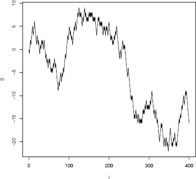
> which(S == 0)
[1] 1 3 27 29 31 37 41 95 225 229 233 237 239 241
The value of Sn can be determined by the partial random walk starting at the most recent time the process returned to 0.
If the state of the symmetric random walk Sn at time n is required, but not the history up to time n, then for large n it may be more efficient to generate Sn as follows.
Assume that S0 = 0 is the initial state of the process. If the process has returned to the origin before time n, then to generate Sn we can ignore the past history up until the time the process most recently hit 0. Let T be the time until the first return to the origin. Then to generate Sn, one can simplify the problem by first generating the waiting times T until the total time first exceeds n. Then starting from the last return to the origin before time n, generate the increments Xi and sum them.
Algorithm to simulate the state Sn of a symmetric random walk
The following algorithm is adapted from [69, XIV.6].
Let Wj be the waiting time until the jth return to the origin.
- Set W1 = 0.
- For j = 1, 2,... while Wj ≤ n:
- Generate a random Tj from the distribution of the time until the first return to 0.
- Set Wj = T1 + ··· + Tj.
- Set t0 = Wj — Tj (time of last return to 0 in time n.)
- Set s1 = 0.
- Generate the increments from time t0 + 1 until time n:
For i = 1,2,...,n — t0- Generate a random increment xi ~ P(X = ±1) = 1/2.
- Set si = x1 + · · · + xi.
- If si = 0 reset the counter to i = 1 (another return to 0 is not accepted, so reject this partial random walk and generate a new sequence of increments starting again from time t0 + 1.)
- Deliver si.
To implement the algorithm, one needs to provide a generator for T, the time until the next return of the process to 0. The probability distribution of T [69, Thm. 6.1] is given by
Example 3.27 (Generator for the time until return to origin)
An efficient algorithm for generating from the distribution T is given by Devroye [69, p. 754]. Here we will apply an inefficient version that is easily implemented in R. Notice that p2n equals 1/(2n) times the probability P(X = n−1) where X ~ Binomial (2n − 2, p = 1/2).
The following methods are equivalent.
#compute the probabilities directly
n <- 1:10000
p2n <- exp(lgamma(2*n-1)
- log(n) - (2*n-1)*log(2) - 2*lgamma(n))
#or compute using dbinom
P2n <- (.5/n) * dbinom(n-1, size = 2*n-2, prob = 0.5)
Recall that if X is a discrete random variable and
are the points of discontinuity of FX(x), then the inverse transformation is , where . Therefore, a generator can be written for values of T up to 20000 using the probability vector computed above.
pP2n <- cumsum(P2n)
#for example, to generate one T
u <- runif(1)
Tj <- 2 * (1 + sum(u > pP2n))
Here are two examples to illustrate the method of looking up the solution in the probability vector.
#first part of pP2n
[1] 0.5000000 0.6250000 0.6875000 0.7265625 0.7539062 0.7744141
In the first example u = 0.6612458 and the first return to the origin occurs at time n = 6, and in the second example u = 0.5313384 and the next return to the 0 occurs at time n = 4 after the first return to 0. Thus the second return to the origin occurs at time 10. (The case u > max(pP2n) must be handled separately.)
Suppose now that n is given and we need to compute the time of the last return to 0 in (0, n].
n <- 200
sumT <- 0
while (sumT <= n) {
u <- runif(1)
s <- sum(u > pP2n)
if (s == length(pP2n)) warning("T is truncated")
Tj <- 2 * (1 + s)
#print(c(Tj, sumT))
sumT <- sumT + Tj
}
sumT - Tj
In case the random uniform exceeds the maximal value in the cdf vector pP2n, a warning is issued. Here instead of issuing a warning, one could append to the vector and return a valid T. We leave that as an exercise. A better algorithm is suggested by Devroye [69, p. 754]. One run of the simulation above generates the times 110, 128, 162, 164, 166, 168, and 210 that the process visits 0 (uncomment the print statement to print the times). Therefore the last visit to 0 before n = 200 is at time 168.
Finally, S200 can be generated by simulating a symmetric random walk starting from S168 = 0 for t = 169, ... , 200 (rejecting the partial random walk if it hits 0).
Packages and Further Reading
General references on discrete event simulation and simulation of stochastic processes include Banks et al. [18], Devroye [69], and Fishman [95]. Algorithms for generating random tours in general are discussed by Fishman [94, Ch. 5]. Also see Cornuejols and Tütüncü [53] on related optimization methods.
Ross [234, Ch. 10] has a nice introduction to Brownian Motion, starting with the interpretation of Brownian Motion as the limit of random walks. For a more theoretical treatment see Durrett [77, Ch. 7].
See Franklin [98] for simulation of Gaussian processes. Functions to simulate long memory time series processes, including fractional Brownian motion are available in the R package fSeries (see e.g. fbmSim) [299] and sde [149]. The FracSim package [65, 66] implements methods for simulation of multi-fractional Lévy motions. Also see Coeurjolly [51] for a bibliographical and comparative study on simulation and identification of fractional Brownian motion.
References on the general subject of methods for generating random variates from specified probability distributions have been given in Section 3.1.
Exercises
3.1 Write a function that will generate and return a random sample of size n from the two-parameter exponential distribution Exp(λ, η) for arbitrary n, λ, and η. (See Examples 2.3 and 2.6.) Generate a large sample from Exp(λ, η) and compare the sample quantiles with the theoretical quantiles.
3.2 The standard Laplace distribution has density Use the inverse transform method to generate a random sample of size 1000 from this distribution. Use one of the methods shown in this chapter to compare the generated sample to the target distribution.
3.3 The Pareto(a, b) distribution has cdf
Derive the probability inverse transformation F−1(U) and use the inverse transform method to simulate a random sample from the Pareto(2, 2) distribution. Graph the density histogram of the sample with the Pareto(2, 2) density superimposed for comparison.
3.4 The Rayleigh density [156, Ch. 18] is
Develop an algorithm to generate random samples from a Rayleigh(σ) distribution. Generate Rayleigh(σ) samples for several choices of σ > 0 and check that the mode of the generated samples is close to the theoretical mode σ (check the histogram).
3.5 A discrete random variable X has probability mass function
Use the inverse transform method to generate a random sample of size 1000 from the distribution of X. Construct a relative frequency table and compare the empirical with the theoretical probabilities. Repeat using the R sample function.
3.6 Prove that the accepted variates generated by the acceptance-rejection sampling algorithm are a random sample from the target density fX.
3.7 Write a function to generate a random sample of size n from the Beta(a, b) distribution by the acceptance-rejection method. Generate a random sample of size 1000 from the Beta(3,2) distribution. Graph the histogram of the sample with the theoretical Beta(3,2) density superimposed.
3.8 Write a function to generate random variates from a Lognormal(μ, σ) distribution using a transformation method, and generate a random sample of size 1000. Compare the histogram with the lognormal density curve given by the dlnorm function in R.
3.9 The rescaled Epanechnikov kernel [85] is a symmetric density function
Devroye and Györfi [71, p. 236] give the following algorithm for simulation from this distribution. Generate iid U1, U2, U3 ~ Uniform(−1, 1). If |U3| ≥ |U2| and |U3| ≥ |U1|, deliver U2; otherwise deliver U3. Write a function to generate random variates from fe, and construct the histogram density estimate of a large simulated random sample.
3.10 Prove that the algorithm given in Exercise 3.9 generates variates from the density fe (3.10).
3.11 Generate a random sample of size 1000 from a normal location mixture. The components of the mixture have N(0,1) and N(3,1) distributions with mixing probabilities p1 and p2 = 1 − p1. Graph the histogram of the sample with density superimposed, for p1 = 0.75. Repeat with different values for p1 and observe whether the empirical distribution of the mixture appears to be bimodal. Make a conjecture about the values of p1 that produce bimodal mixtures.
3.12 Simulate a continuous Exponential-Gamma mixture. Suppose that the rate parameter A has Gamma(r, β) distribution and Y has Exp(A) distribution. That is, (Y |Λ = λ) ~ fY (y|λ) = λe−λy. Generate 1000 random observations from this mixture with r = 4 and β = 2.
3.13 It can be shown that the mixture in Exercise 3.12 has a Pareto distribution with cdf
(This is an alternative parameterization of the Pareto cdf given in Exercise 3.3.) Generate 1000 random observations from the mixture with r = 4 and β = 2. Compare the empirical and theoretical (Pareto) distributions by graphing the density histogram of the sample and superimposing the Pareto density curve.
3.14 Generate 200 random observations from the 3-dimensional multivariate normal distribution having mean vector μ = (0, 1, 2) and covariance matrix
using the Choleski factorization method. Use the R pairs plot to graph an array of scatter plots for each pair of variables. For each pair of variables, (visually) check that the location and correlation approximately agree with the theoretical parameters of the corresponding bivariate normal distribution.
3.15 Write a function that will standardize a multivariate normal sample for arbitrary n and d. That is, transform the sample so that the sample mean vector is zero and sample covariance is the identity matrix. To check your results, generate multivariate normal samples and print the sample mean vector and covariance matrix before and after standardization.
3.16 Efron and Tibshirani discuss the scor (bootstrap) test score data on 88 students who took examinations in five subjects [84, Table 7.1], [188, Table 1.2.1]. Each row of the data frame is a set of scores (xi1, ... , xi5) for the ith student. Standardize the scores by type of exam. That is, standardize the bivariate samples (X1, X2) (closed book) and the trivariate samples (X3, X4, X5) (open book). Compute the covariance matrix of the transformed sample of test scores.
3.17 Compare the performance of the Beta generator of Exercise 3.7, Example 3.8 and the R generator rbeta. Fix the parameters a = 2, b = 2 and time each generator on 1000 iterations with sample size 5000. (See Example 3.19.) Are the results different for different choices of a and b?
3.18 Write a function to generate a random sample from a (Wishart) distribution for n > d + 1 ≥ 1, based on Bartlett’s decomposition.
3.19 Suppose that A and B each start with a stake of $10, and bet $1 on consecutive coin flips. The game ends when either one of the players has all the money. Let Sn be the fortune of player A at time n. Then {Sn, n ≥ 0} is a symmetric random walk with absorbing barriers at 0 and 20. Simulate a realization of the process {Sn, n ≥ 0} and plot Sn vs the time index from time 0 until a barrier is reached.
3.20 A compound Poisson process is a stochastic process {X(t), t ≥ 0} that can be represented as the random sum where {N(t), t ≥ 0} is a Poisson process and Y1, Y2,... are iid and independent of {N(t), t ≥ 0}. Write a program to simulate a compound Poisson(λ)–Gamma process (Y has a Gamma distribution). Estimate the mean and the variance of X(10) for several choices of the parameters and compare with the theoretical values. Hint: Show that E[X(t)] = λtE[Y1] and Var(X(t)) = λtE[Y12].
3.21 A nonhomogeneous Poisson process has mean value function m(t) = t2 + 2t, t > 0. Determine the intensity function λ(t) of the process, and write a program to simulate the process on the interval [4, 5]. Compute the probability distribution of N(5)−N(4), and compare it to the empirical estimate obtained by replicating the simulation.