
Chapter 6. Building a data model
In this chapter, David moves to the next level in Microsoft Power BI usage. We are probably cheating a bit now, but we wanted this book to show you what Power BI can do for you when you master it, not just demonstrate its basic features. To do that, we presume that David—encouraged by the good results so far—spent some time learning the basics of data modeling and the DAX language. Having learned more details about Power BI, he begins again building the budgeting solution, but this time he can trust his better knowledge of the tools.
David loads the sales in the previous years, but unlike the last time, he does not use the view that Karin, the database administrator at Contoso, created for him. Instead, he uses more basic views, on top of the Contoso data warehouse, that provide data in a more fragmented way. There is a table containing information on the stores, one with the sales data, one for the date, and, lastly, a table of the products themselves. Using this information, he builds a first sales analysis project. Finally, he adds the budget information from the Microsoft Excel workbook and writes some DAX code to prepare the dashboards.
We will not discuss in detail all of the formulas and intricacies of the code and the data model; it’s not realistic to expect you to learn how to perform these operations by reading one chapter. Our goal is to build the full project together (remember, you can replicate it by using the companion content). If you like the final project, you will probably be better motivated to proceed further with your study and follow David’s path in learning data modeling and DAX.
Loading individual tables
Recall from Chapter 3 that David needed to speak with Karin to gain access to the Microsoft SQL Server database containing a view that returns sales for the past three years. David learned that he can perform an analysis on sales in a better way if—instead of using Karin’s view—he loads the data from the original tables where Karin stores Contoso information. So, he arranges a meeting with Karin to gather more information about the internal structure of the Contoso data warehouse.
Karin explains to him that the database is organized in tables that he can access by using individual views (one per table). There is a table for each business entity of Contoso’s business:
• Products This table contains information about the products sold by Contoso.
• Sales This one contains detailed sales, one row for each individual sale.
• Stores This table has information about the stores where the sales were transacted.
• Date This is a helper table that contains the calendar. David learned in a Business Intelligence class that such a table is of paramount importance when building a good data model.
Karin gives David access to the views so that he can load the granular information. David decides to begin again from scratch, so he opens Power BI Desktop and loads these tables into a new model, following the same procedure he did to load the Sales2015 view. The only difference is this time he loads four tables at once, as shown in Figure 6-1.

Instead of loading the tables directly from the Navigator dialog box, you’ll find it more convenient to click the Edit Queries button (on the Home tab of the ribbon, in the External Data group) to open Query Editor and then change the names of the tables, removing the ContosoBi prefix. In fact, as you might remember, Query Editor names them ContosoBi.Sales instead of the more readable Sales.
After you close Query Editor, Power BI Desktop loads the table in the model and automatically creates some relationships among them. The Power BI Desktop algorithm that detects relationships is not perfect, and, in fact, it did not detect all of the relationships between the tables.
To follow along and catch up to this point, open Power BI Desktop and then open the companion content file for Chapter 6: Budget – Start.pbix. On the navigation bar, David clicks the Relationship View icon. He then sees the model illustrated in Figure 6-2 and notices that a relationship wasn’t created between the Date and Sales tables.

Figure 6-2: The Power BI Desktop relationship detector did not find the relationship between Sales and Date.
This is not an issue; you can easily create the relationship between Date and Sales by dragging DateKey from the Sales table to DateKey in the Date table to link the two tables with the correct relationship. The final data model is presented in Figure 6-3. (Note that your view of the data models might be different; for example, the Date table might be to the left of Sales, not below it.)

Figure 6-3: The data model structure is a very simple schema, with Sales in the middle and the other tables around it.
Implementing measures
The model, as it is, still requires some adjustments. First, David hides all of the columns that should not be visible when creating reports. He does this by going to Report View, selecting the table columns, right-clicking one, and then clicking Hide. David hides all of the keys and the columns that would be misleading if they were summed straight.
For example, the Sales table contains Quantity and Net Price. By default, Power BI offers to summarize Net Price by summing the values. In reality, this would be wrong because summing the price would not take into consideration the quantity sold.
Note
The Sales table in the Budget – Start.pbix file is hidden by default because all of its columns are hidden. To make it visible, in Data View, right-click the table, and then, on the shortcut menu that opens, click Unhide All.
The default summarization used by Power BI works perfectly well when you have a simple data model. But, as soon as you begin loading data from relational databases for which numbers are not stored in such a way as to be used in Excel workbooks, you need to stop using default summarization and begin writing DAX measures, instead. Measures, in DAX parlance, are scripts that you write using DAX-specific syntax. By using measures, you can author your own code and produce much more powerful data models.
David creates a simple measure to compute the Sales Amount. In Report View, in the Fields pane, David right-clicks the Sales table and then clicks New Measure. In the formula bar above the canvas in the middle pane, he replaces “Measure =” with the following code:
Sales Amount = SUMX ( Sales, Sales[Quantity] * Sales[Unit Price] )
This measure alone is already extremely powerful. In fact, because David is now loading data directly from the data warehouse, he can slice sales by using any of the available columns, not just those that were present in the single view he was using before. For example, now the Product table contains Category and Subcategory, which are useful for performing an analysis of sales in different countries/regions, with a report such as the one depicted in Figure 6-4.

Analysis of sales in previous years becomes more interesting as soon as you have more columns available. The report shows the relative contribution of different brands to the Computers category (notice how the Computers category is selected in the lower-left bar chart in Figure 6-4), whereas the line chart shows the behavior of sales over time. Different years are highlighted by different line colors. Using this tool, David can find an answer to different questions, like what is the reason for the peak in September 2013.
Creating calculated columns
Having more power typically raises the requirements of the data model. As an example, consider the line chart: having the sales of the three years with different lines might be useful for a comparison of different years; however, if you want to analyze the behavior of sales over the three years, it would be much better to show a single line that spans all of the years.
The problem is that the Date table contains the month name, and you can easily use it as we did in Figure 6-4, but if you remove the year from the legend, you get sales divided by month, not by month and year, as shown in Figure 6-5.

David needs a column containing both year and month at the same time. Such a column is not available in the original database. Fortunately, he has two different options to create this column: he can use Query Editor to add the column to the Date query, or he can create a calculated column.
In Chapter 4, you learned how to use Query Editor to generate new columns; let’s use this as an opportunity to learn how to use calculated columns. To create a new column in a table, on the Power BI Desktop ribbon, on the Modeling tab, click New Column, as indicated in Figure 6-6.

You can add these two columns to the Date table by typing the following measures in the formula bar above the table:
Month Year = FORMAT ( 'Date'[Date], "mmm YY" )
Month Year Number = 'Date'[Year] * 100 + MONTH ( 'Date'[Date] )
The first column contains a shortened version of month and year (we keep it short, to make it suitable for the line chart), whereas the second column is used to sort the first one, using the Sort By Column feature we already discussed.
If you now replace the Month Name with the Month Year as the axis of the line chart, the visualization is exactly what you want, showing the behavior of sales over three years, as you can see in Figure 6-7.

Figure 6-7: Using a calculated column for the axis of the line chart leads to the desired visualization.
When building reports, you will typically need a calculated column to make the visualization look perfect. Sometimes the descriptions are too large. In other cases, such as this one, you need a column representing a specific behavior. Power BI is an environment in which you model the data while having the visualization in mind as the final goal.
Improving the report by using measures
When you use calculated columns and measures to perform analyses, you’re limited only by your imagination. For example, with a few calculations you can easily build a report like the one shown in Figure 6-8, which shows a bubble chart with the number of products versus the margin divided by category, where the size of each bubble is the amount sold.

Figure 6-8: A bubble chart shows a large amount of information in a single chart, and they are gorgeous when used with visual interaction and automatic filtering.
The measures needed to build the report are very simple:
NumOfProducts = COUNTROWS ( 'Product' )
Gross Margin = SUMX ( Sales, Sales[Quantity] * ( Sales[Unit Price] - Sales[Unit Cost] ) )
NumOfProducts simply counts the number of products and gives an idea of how many articles are in the portfolio, whereas Gross Margin computes the gross margin of sales by subtracting the cost from the unit price before multiplying that value by the quantity.
Note
As you have seen so far, we are not explaining how to write the DAX code. The goal of this chapter is not to teach DAX; a short chapter in a short book would not properly address the complexity of the language. Our goal here is to show you what you can do as soon as you begin learning the basics of data modeling and DAX coding. Incredible analytical power awaits you when you complete your journey learning DAX, so hurry and start learning it today. In the meantime, we will move on with more complex DAX code and present some more scenarios that you can solve by writing simple formulas.
Integrating budget information
So far, David is excited about the power of his analytical tool; so much so, in fact, that he’s forgotten that the task is about budgeting, not sales analysis. This is one of the major drawbacks of using Power BI: it is so much fun to dive into data and analyze it that you might become lost in evocative reports. Now it’s time to get back to business and integrate the budget information.
Loading the budget information from Excel is straightforward, and David has already used the technique. But a problem arises as soon as he looks at the data model. The new table containing the budget does not have any relationship with the other tables, as you can see in Figure 6-9.

This time, it’s not an issue of Power BI failing to detect the relationship, which earlier David was able to correct by using a simple drag-and-drop technique to establish a relationship. In this instance, the relationship cannot be created this way. In fact, when he tries to drag CountryRegion from the Budget table to the Store table, he sees the error shown in Figure 6-10.

Figure 6-10: Trying to create a relationship between the Budget and Store tables leads to this error.
The error message suggests that an intermediate table might help solve the problem. But, before solving the issue, it’s worth taking a few moments to understand it better.
You can create a relationship between two tables if the column you use to create the relationship is a key in the destination table. You can create a relationship between the Sales and Date tables based on the DateKey column because DateKey has a different value for each row in Date. Having a different value for each row is the requisite for a column to be a key. In fact, when you have a given date, you can uniquely identify the entire row in Date. In the model with Budget, CountryRegion is neither a key in the Budget table, nor in Store. Thus, you cannot create such a relationship.
There are multiple ways to solve this problem, based on the model or on an advanced usage of the DAX language. The solution based on the model is somewhat easier to learn and, by the way, it is the way suggested by the error message.
If you create a table containing all the possible values of CountryRegion, CountryRegion becomes a key for that table. At that point, you are able to create the relationships between Budget and Store.
You can build a table containing the possible values of CountryRegion by using Query Editor, as you did in Chapter 4, or by adopting a new technique: a calculated table. Calculated tables are tables computed using the DAX language that you can store in the model and use as any other table. To create a calculated table, on the Power BI ribbon, on the Modeling tab, click New Table, and then, in the formula bar, type the following DAX expression:
CountryRegions =
SUMMARIZE (
UNION (
DISTINCT ( Budget[CountryRegion] ),
DISTINCT ( Store[CountryRegion] )
),
[CountryRegion]
)
Figure 6-11 shows the resulting table.

Let’s return to see how David is faring. To create the table, he takes the distinct values of both the Budget[CountryRegion] and Store[CountryRegion] columns, forms a union with the partial results, and finally the Summarize function returns a summary table of the CountryRegion column. In this way, all the possible values will be represented in the resulting table, either referenced by the Budget or Store tables.
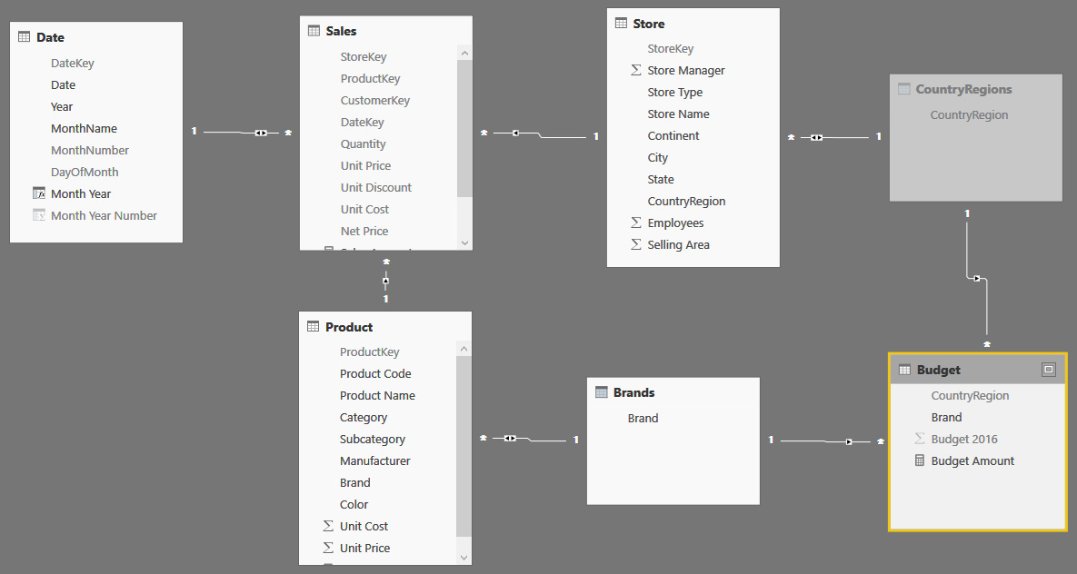
Now, David has the intermediate table that the error message in Figure 6-10 suggested to him. He can create one relationship between Store and CountryRegions, and another one between Budget and CountryRegions, completing the model. The table is a technical table, which is useful only to propagate the filter from Store to the Budget. Figure 6-12 presents the data model with the new table in place.

From a technical point of view, David created a many-to-many relationship between the Budget and Store tables, using CountryRegions as the bridge table between them. To test that the model works well, he creates the following simple measure that returns the sum of the budget:
Budget Amount = SUM ( Budget[Budget 2016] )
You can project this measure on a simple report containing CountryRegion, the value of budget, and the value of sales. Now, CountryRegion correctly slices both Sales Amount and Budget Amount, as illustrated in Figure 6-13.

The first problem, here, is that the report is not showing meaningful numbers. In fact, because there is no filter on the year, it is accumulating sales over all available years and comparing them with the budget, which contains forecasts for 2016 only. You can easily solve the issue by creating the following measure that computes the sales amount for only 2015:
Sales 2015 = CALCULATE ( [Sales Amount], 'Date'[Year] = 2015 )
By replacing Sales Amount with Sales 2015 in the report, the numbers can be compared, as demonstrated in Figure 6-14.

You also need to apply the same technique to the other column available in budget, which is Brand. The DAX code is very similar to the previous example; you have only to change the column names to obtain the list of all the possible brands:
Brands =
SUMMARIZE (
UNION (
DISTINCT ( Budget[Brand] ),
DISTINCT ( Product[Brand] )
),
[Brand]
)
So far, so good. The next step hides a problem that—again—requires a bit of theory to be explained.
When you create the relationships between Product, Budget, and Brands, you end up with a model like the one depicted in Figure 6-15, wherein the relationship between Budget and Brands has been created but remained inactive (this is because it was the last one we created—by following a different order in the creation of relationships, you might obtain the relationship between Product and Brands as an inactive one).

Figure 6-15: Among the many relationships, the one between Brands and Budget is inactive, signified by the dashed connector line between them.
What is an inactive relationship? It is a relationship that is present in the model but not used in the automatic filtering of values. Why did Power BI Desktop deactivate the last relationship we created? Because if it did not deactivate it, we would end up with an ambiguous model.
With the inactive relationship, filtering does not happen in the correct way. In fact, if you build a report using countries/regions and brands, the result is wrong, as demonstrated in Figure 6-16.

Figure 6-16: Slicing by Brand does not produce a meaningful result (all of the values are repeated) because the underlying relationship is inactive.
An ambiguous model is a data model within which there are multiple paths linking two tables because all of the relationships are set as bidirectional (that is, the filter applies in both directions). (Note that you can tell when a relationship is bidirectional because there are two small arrows on the connector line, facing both directions.) So, where is the ambiguity? There are many here. For example, if you start from Product (see Figure 6-15), you can reach Budget following the bottom chain Product/Brands/Budget or the upper chain Product/Sales/Store/CountryRegion/Budget. If all of the relationships remained active, both would be legal paths, and you would end up with ambiguity.
You can solve ambiguity in most cases by just preventing the path from being traversed, but still maintaining the model features. For example, in the model examined, there is no need to make Sales filter Store and Sales filter Product. It is enough that the opposite direction works in both cases; that is, you can have both the Store and Product tables filter Sales. To perform this, you can double-click a relationship (the connector line between Sales and Store, for example), which opens the Edit Relationship dialog box, as shown in Figure 6-17.

Figure 6-17: In the Edit Relationship dialog box, you can configure many properties of a relationship.
To disable bidirectional filtering, you must set the Cross Filter Direction to Single. You should do this to several relationships: the one between Sales and Store, the one between Sales and Product, and to the two linking Budget with CountryRegions and Brands. The final model is represented in Figure 6-18.
After you remove ambiguity from the model and activate the correct set of relationships, the model works fine. You can test it by building a simple matrix that shows both Brand and CountryRegion now filtering the budget correctly, as illustrated in Figure 6-19.

Reallocating the budget
Budget numbers are correct as long as you slice by brand or by country/region, which is the granularity at which the budget is defined. However, if you add a column that is not a part of the Budget table (for example, you can slice by Country/Region and Color), the result will be wrong. Figure 6-20 shows that values for Black and Silver colors in United States have the same value as the grand total of all the colors in United States.

In reality, it is not that the number is wrong; it’s just that it is very difficult to understand what it is computing. For example, the value in the cell at the intersection of United States and Black shows the sum of the budget in the United States for all the brands that have at least one product of the color black. Because some colors, like Black and Silver, are present for every brand, these rows show the same value of the grand total.
The number shown is clearly not what you would like to see. Intuitively, you would like to see the budget related to only Black products in the United States. However, with the data model we have so far, this is not what you obtain.
The problem is that the budget for black products (or any other color, for instance) is not available in the source workbook. There, you only have the budget for all the products of the same brand. Nevertheless, even if the number is not there, you can compute it by using a technique that is similar to the easy one David used at the beginning of this book (you might remember that David sliced the budget by month and then simply divided that value by 12).
To better understand the technique, let’s begin with the report presented in Figure 6-21, which shows budget and sales in a matrix, and a chart used to filter and show only Contoso’s data.

Figure 6-21: The report shows Budget and Sales 2015 sliced by color for the individual brand, Contoso.
What is the budget value for Black? You can take the grand total (which is 239,500.00) and multiply it by an allocation factor computed by dividing sales of Black in 2015 (49,592.00) by the grand total of sales (228,978.00). Thus, the correction factor is 0.2165, and the value to display is 51,781.
Using this technique, you allocate the budget based on sales in the previous year. This time you take into account the correct seasonality and any other factors that made higher or lower sales for a specific color, category, or subcategory.
The budget has a granularity of brand and country/region. If you focus only on the Brand at the moment, you can compute the allocation factor by using the following measure:
AllocationFactor =
DIVIDE (
[Sales 2015],
CALCULATE ( [Sales 2015], ALLEXCEPT ( 'Product', 'Product'[Brand] ) )
)
Figure 6-22 shows the value of such a measure formatted as a percentage.

Figure 6-22: The allocation factor is the percentage to compute Budget Amount for when you analyze the budget at a lower granularity.
At this point, you can modify the code of Budget Amount, taking into account the allocation factor.
Budget Amount = SUM ( Budget[Budget 2016] ) * [AllocationFactor]
The result, which is shown in Figure 6-23, shows that now the budget is correctly sliced by Color, even if the original budget was not.

So far, we have focused only on the Brand, which is an attribute of the Product table. Alas, the budget also is defined at the CountryRegion level, and we need to take this into account. You need to consider the CountryRegion when computing the allocation factor, similarly to what you did for the brand before. These are the final versions of the formulas to use:
AllocationFactor =
DIVIDE (
[Sales 2015],
CALCULATE (
[Sales 2015],
ALLEXCEPT ( 'Product', 'Product'[Brand] ),
ALLEXCEPT( Store, Store[CountryRegion] ),
ALL ( Date )
)
)
Budget Amount = SUM ( Budget[Budget 2016] ) * [AllocationFactor]
Figure 6-24 demonstrates that the allocation is performed against 2015. Notice in the same chart on the right, the measures Budget Amount, Sales 2015, and Sales 2014. Budget follows the same distribution of Sales 2015 and ignores Sales 2014, which has a different distribution of numbers.

Figure 6-24: Distribution of Budget Amount is identical to Sales 2015 and different from Sales 2014.
Conclusions
As we said in the introduction, in this chapter we cheated a bit. We did not want to show you another step-by-step guide to implement another dashboard. Instead, we wanted to give you a sneak preview of the capabilities of Power BI Desktop when you uncover the most advanced tools, namely:
• Building a model When you begin loading the raw tables from the SQL Server database, instead of predefined queries with aggregated values, you can perform much more powerful analyses. At the same time, you are responsible for handling the data model by yourself. Power BI Desktop offers you all the tools required to build a complex data model.
• The DAX language DAX is your best friend in the process of analyzing data. In this chapter, we used it to create calculated columns, measures, and calculated tables. This book is not the proper venue for explaining how DAX works; that would fill an entire book by itself. If you are interested in learning more about DAX, check out our book The Definitive Guide to DAX (Microsoft Press, 2015).
• Building columns for specific charts Sometimes, you need a column for an individual chart. There is nothing wrong with doing this; you can just build it.
By using some basic skills, you can take Power BI from a simple reporting tool to what it really is: an extremely powerful modeling tool with which you can build gorgeous analyses on top of your data.