
Chapter 3
Customizing Excel
Performing a Simple Ribbon Modification
Sharing Customizations with Others
Questions About Ribbon Customization
The Excel Options dialog box offers dozens of changes you can make in Excel. This chapter walks you through examples of customizing the ribbon and discusses some of the important option settings available in Excel.
Performing a Simple Ribbon Modification
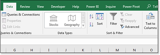
Suppose that you generally like the ribbon, but there is one icon that seems to be missing. You can add icons to the ribbon to make it customized to your preference. If you feel the Data tab would be perfect with the addition of a pivot table icon, you can add it (see Figure 3.1).
To add the pivot table command to the Data tab, follow these steps:
Right-click the ribbon and select Customize The Ribbon.
In the right list box, expand the Data tab by clicking the + sign next to Data.
Click the Sort & Filter entry in the right list box. The new group will go after this entry.
Click the New Group button at the bottom of the right list box. A New Group (Custom) item appears after Sort & Filter, as shown in Figure 3.2.
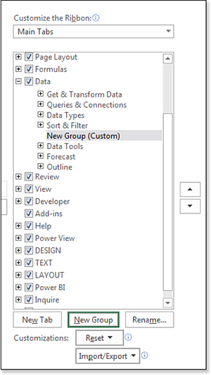
Figure 3.2 Commands have to be added to a new group. While the New Group is selected, click the Rename button at the bottom of the list box. The Rename dialog box appears.
The Rename dialog box offers to let you choose an icon and specify a name for the group. The icon is shown only when the Excel window is too small to display the whole group. Choose any icon and type a display name of
Pivot. Click OK.The left list box shows the popular commands. You could change Popular Commands to All Commands and scroll through 2,400 commands. However, in this case, the commands you want are on the Insert tab. Choose All Tabs from the top-left drop-down menu. Expand the Insert tab, and then expand Tables. Click PivotTable in the left list box. Click the Add button in the center of the dialog box to add PivotTable to the new custom Pivot group on the ribbon. Excel automatically advances to the next icon of Recommended PivotTables. Click Add again.
In the drop-down menu above the left list box, select All Commands. The left list box changes to show an alphabetical list of all commands.
Scroll through the left list box until you find PivotTable And PivotChart Wizard. This is the obscure entry point to create Multiple Consolidation Range pivot tables. Select that item in the left list box. Click Add. At this point, the right side of the dialog box should look like Figure 3.3.
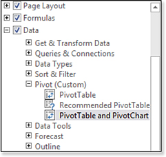
Figure 3.3 Three new icons have been added to a new custom group on the Data tab. Click OK.
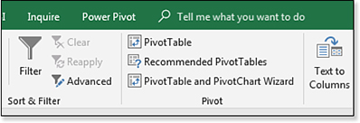
Figure 3.4 shows the new group in the Data tab of the ribbon.
Adding a New Ribbon Tab
To add a new ribbon tab, follow these basic steps:
Right-click the ribbon and select Customize The Ribbon.
Click New Tab and rename the tab.
Add New Group(s) to the new tab.
Add commands to the new groups.
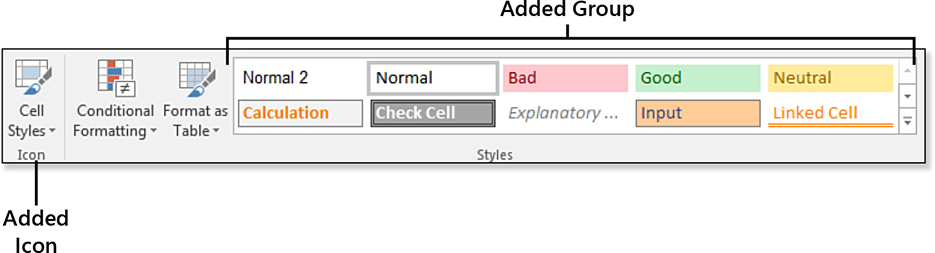
As you go through the steps to add a new ribbon tab, you will discover how absolutely limiting the ribbon customizations are. You have no control over which items appear with large icons and which appear with small icons. This applies even to galleries. If you add the Cell Styles gallery to a group on the ribbon, it always appears as an icon instead of a gallery, even if it is the only thing on the entire ribbon tab (see the left icon in Figure 3.5). The workaround is to add an entire built-in group to the tab. On the right of Figure 3.5, the entire Styles group was added. The Cell Styles gallery is now allowed to appear as a gallery.
Troubleshooting
When customizing the ribbon using this interface, you cannot control which icons appear large and which appear small in the ribbon.
The Excel ribbon contains a logical mix of large icons for important features and small icons for minor features. If you would like to create a new group, you cannot control which icons will be small and which will be large.
You can either learn RibbonML or use a third-party tool such as Ribbon Commander to create custom ribbon tabs. Try a free trial of Ribbon Commander at https://mrx.cl/ribboncommander.
Sharing Customizations with Others
If you have developed the perfect ribbon customization and you want everyone in your department to have the same customization, you can export all the ribbon customizations.
To export the changes, follow these steps:
Right-click the ribbon and select Customize The Ribbon.
Below the right list box, select Import/Export, Export All Customizations.
Browse to a folder and provide a name for the customization file. The file type will be .exportedUI. Click OK.
In Windows Explorer, find the .exportedUI file. Copy it to a co-worker’s computer.
On the co-worker’s computer, repeat step 1. In step 2, select Import Customization File. Find the file and click OK.
Note
This is an all-or-nothing proposition. You cannot export your changes to one custom tab without exporting your changes to the Data and Home tabs.
Questions About Ribbon Customization
Can the customizations apply only to a certain workbook?
No. The Customize The Ribbon command in Excel 2019 applies to all workbooks.
Can I reset my customizations and go back to the original ribbon?
Right-click the ribbon and select Customize The Ribbon. Below the right list box, select Reset, Reset All Customizations.
How can I get complete control over the ribbon?
Learn RibbonX and write some VBA to build your own ribbon.
![]() For more information on building your own ribbon, see RibbonX: Customizing the Office 2007 Ribbon, by Robert Martin, Ken Puls, and Teresa Hennig (Wiley, ISBN 0470191112).
For more information on building your own ribbon, see RibbonX: Customizing the Office 2007 Ribbon, by Robert Martin, Ken Puls, and Teresa Hennig (Wiley, ISBN 0470191112).
These ribbon customizations are really lacking. Is there another option that doesn’t require me to write a program?
Yes, some third-party ribbon customization programs are available. For example, check out a free one from Excel MVP Andy Pope at www.andypope.info/vba/ribboneditor.htm.
Using the Excel Options Dialog Box
Open the File menu and select Options from the left navigation pane to open the Excel Options dialog box. The dialog box has categories for General, Formulas, Data, Proofing, Save, Language, Ease Of Access, Advanced, Customize Ribbon, Quick Access Toolbar, Add-Ins, and Trust Center. The Trust Center leads to another 12 categories.
To the Excel team’s credit, they tried to move the top options to the General category. Beyond those 15 settings, though, are hundreds of settings spread throughout 21 categories in the Excel Options and Trust Center. Table 3.1 gives you a top-level view of where to start looking for settings.
Table 3.1 Excel Options Dialog Box Settings
Category |
Types of Settings |
|---|---|
General |
The most commonly used settings, such as user interface settings, the default font for new workbooks, number of sheets in a new workbook, customer name, and Start screen. |
Formulas |
All options for controlling calculation, error-checking rules, and formula settings. Note that options for multithreaded calculations are currently considered obscure enough to be on the Advanced tab rather than on the Formulas Tab. |
Data |
The data category is new in 2017. It offers the new Edit Default Layout for pivot tables, several other pivot table options, and then a series of checkboxes to bring back the legacy Get Data categories. When Power Query replaced Get Data on the Data tab of the ribbon, the old legacy icons were removed. |
Proofing |
Spell-check options and a link to the AutoCorrect dialog box. |
Save |
The default method for saving, AutoRecovery settings, legacy colors, and web server options. |
Language |
Choose the editing language, ToolTip language, and Help language. |
Ease of Access |
Options available are Provide Feedback With Sound, Provide Feedback With Animation, Screen Tip Style, and the default document font size. |
Advanced |
All options that Microsoft considers advanced, spread among 14 headings. |
Customize Ribbon |
Icons to customize the ribbon. |
Quick Access Toolbar |
Icons to customize the Quick Access Toolbar (QAT). |
Add-Ins |
A list of available and installed add-ins. New add-ins can be installed from the button at the bottom of this category. |
Trust Center |
Links to the Microsoft Trust Center, with 12 additional categories. |
Getting Help with a Setting
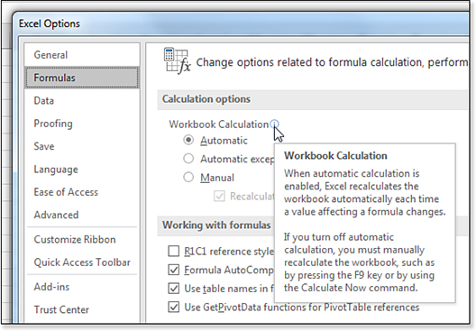
Many settings appear with a small i icon. If you hover the mouse near this icon, Excel displays a super ToolTip for the setting. The ToolTip explains what happens when you choose the setting. It also provides some tips about what you need to be aware of when you turn on the setting. For example, the ToolTip in Figure 3.6 shows information about the calculation settings. It also explains that you should use the F9 key to invoke a manual calculation.
New Options in Excel 2019
Excel 2019 offers several new settings:
Office Intelligent Services is found on the General category. This Office-365 exclusive feature will send up to 250,000 cells of your worksheet to a Microsoft Artificial Intelligence application for analysis. You must opt-in to use this feature in Options and then invoke the feature using the Insights command on the Insert menu.
Enable LinkedIn Features is found in the General category. Microsoft purchased LinkedIn, and they added features to allow LinkedIn profile information to appear in Outlook and Word. There are not any LinkedIn features available in Excel (yet), so you must wonder why they added this option in Excel.
Default PivotTable Layout is found in the new Data category. Change the default layout for all future pivot tables. Several items in the new Data category were moved to the Data category from the Advanced category.
Disable Automatic Grouping Of Date/Time Columns In A Pivot Table is found in the Data category. One of the highly touted features in Excel 2016 was that any date field added to a pivot table would be rolled up to years and months. Some people hated it, and so now there is a checkbox to turn it off.
Show Legacy Data Import Wizards is a series of seven choices in the new Data category. The Power Query tools debuted in Excel 2016 on the Data tab of the ribbon. These tools became so popular, Microsoft decided to remove the old Get External Data group from the ribbon, but some people had specific reasons why they liked the old icons. You can now add those old icons back by choosing From Access, From Web, From Text, From SQL Server, From OData Data Feed, From XML Data Import, or From Data Connection. If you choose something from this area, it will appear hidden on the ribbon. Look in Data, Get Data, Legacy Wizards.
AutoSave OneDrive And SharePoint Online Files By Default On Excel is the first item in the Save category of Excel Options. A small percentage of people need to have many people work in the same workbook at the same time. A large percentage of people who don’t need this feature quickly hated that Excel was saving their file after every change. You can globally turn AutoSave Off or On using this setting. I recommend leaving it off. Then, for the workbooks that you need to edit with other people, you can turn it on.
Show Data Loss Warning When Editing Comma Delimited Files (*.csv) is found in the Save category. Excel used to nag you whenever you opened a file in CSV format. If you did not save the file as XLSX, it would warn you that you are about to lose formulas and formatting. A lot of people were tired of the nagging, and Microsoft turned off the nagging by default. If you need to be nagged, you can turn it back on here.
The ability to save Checked Out files To Server Drafts was removed from the Save category. A Learn More hyperlink in Excel Options explains why.
The Ease Of Access category is new in Excel 2019. You can choose to Provide Feedback With Sound and choose a Modern or Classic sound scheme. The new part is the Modern sound scheme. The annoying Classic Sound Scheme was previously the only choice in the Advanced category. You can turn off Animations. The choice to control if Screen Tips are shown is repeated here from the General category. You can set the Default Font Size used in the document. You can choose to turn off the calculation Function Screen Tips.
Use Pen To Select and Interact By Default is new in the Advanced category. If you prefer using a touchscreen, you can change the default behavior of touch.
Using AutoRecover Options
For many versions, Excel periodically saves a copy of your work every 10 minutes. If your computer crashes, the recovery pane offers to let you open the last AutoRecovered version of the file. This feature is sure to save you from retyping data that might have otherwise been lost.
Another painful situation occurs when you do not save changes and then close Excel. Yes, Excel asks if you want to save changes for each open document, but this question usually pops up at 5:00 p.m. when you are in a hurry to get out of the office. If you are thinking about what you need to do after work and not paying attention to which files are still open, you might click No to the first document and then click No again and again without noticing that the fifth open document was one that should have been saved.
Another scenario involves leaving an Excel file open overnight only to discover that Windows Update decided to restart the computer at 3 a.m. After being burned a dozen times, you can change the behavior of Windows Update to stop doing this. However, if Windows Update closed Excel without saving your documents, you can lose those AutoRecovered documents.
A setting introduced in Excel 2010 has Excel save the last AutoRecovered version of each open file when you close without saving. This setting is on the Save category of Excel Options and is called Keep The Last AutoSaved Version If I Close Without Saving.
Controlling Image Sizes
An Image Size & Quality section appears in the Advanced category. Most people add a photo to dress up the cover page of a document. However, you probably don’t need an 8-megapixel image being saved in the workbook. By default, Excel compresses the image before saving the file. You can control the target output size using the drop-down menu in Excel options. Choices include 96ppi, 150ppi, and 220ppi. The 96ppi setting will look fine on your display. Use 220ppi for images you will print. If you want to keep your images at the original size, you can select the Do Not Compress Images In File setting.
You should also understand the Discard Editing Data check box. Suppose that you insert an image in your workbook and then crop out part of the photograph. If you do not enable Discard Editing Data, someone else can come along and uncrop your photo. This can be an embarrassing situation—just ask the former TechTV co-host who discovered certain bits of photographs were still hanging around after she cropped them out.
Working with Protected View for Files Originating from the Internet
Starting in Excel 2010, files from the Internet or Outlook initially open in protected mode. This mode gives you a chance to look at the workbook and formulas without having anything malicious happen. Unfortunately, you cannot view the macro code while the workbook is in protected view.
If you only want to view or print the workbook, protected mode works great. One statistic says that 40% of the time, people simply open a document and never make changes to it.
After you click Enable Editing, Excel will skip protected mode the next time you open the file.
Working with Trusted Document Settings
By default, Excel warns you about all sorts of things. If you open a workbook with macros, links, external data connections, or even the new WEBSERVICE function, a message bar appears above the worksheet to let you know that Excel disabled those “threats.”
If you declare a folder on your hard drive to be a trusted folder, you can open those documents without Excel warning you about the items. Visit File, Options, Trust Center, Trust Center Settings, Trusted Locations to set up a trusted folder.
Starting in Excel 2010, if you open a file from your hard drive and enable the content, Excel automatically enables that content the next time. The inherent problem here is that if you open a file and discover the macros are bad, you will not want those macros to open the next time automatically. There is no way to untrust a single document other than deleting, renaming, or moving it. Instead, you have to go to the Trusted Documents category of the Trust Center where you can choose to clear the entire list of trusted documents.
Options to Consider
Although hundreds of Excel options exist, this section provides a quick review of options that might be helpful to you:
Save File In This Format in the Save category. If you regularly create macros, choose the Excel Macro-Enabled Workbook as the default format type.
Update your Default File Location in the Save tab. Excel always wants to save new documents in your My Documents folder. However, if you always work in the C:AccountingFiles folder, update the default folder to match your preferred location.
Show This Number Of Recent Workbooks has been enhanced dramatically since Excel 2003. Whereas legacy versions of Excel showed up to nine recent workbooks at the bottom of the File menu, Excel 2019 allows you to see up to 50 recent workbooks in the Open category of the File menu. You can change this setting by visiting the Display section of the Advanced category.
Edit Custom Lists has been moved to the Display section of the Advanced category. Custom lists add functionality to the fill handle, allow custom sort orders, and control how fields are displayed in the label area of a pivot table. Type a list in the correct sequence in a worksheet. Edit Custom Lists and click Import. Excel can now automatically extend items from that list, the same as it can extend January into February, March, and so on.
Make Excel look less like Excel by hiding interface elements in the three Display sections of the Advanced category. You can turn off the formula bar, scrollbars, sheet tabs, row and column headers, and gridlines. You can customize the ribbon to remove all main tabs except the File menu. The point is that if you design a model to be used by someone who never uses Excel, the person can open the model, plug in a few numbers, and get the result without having to see the entire Excel interface.
Show A Zero in Cells That Have Zero Value is in the Display Options For This Worksheet section of the Advanced category. Occasionally people want zeros to be displayed as blanks. Although a custom number format of
0;-0;;will do this, you can change the setting globally by clearing this option.Group Dates in the AutoFilter Menu is in the Display Options For This Workbook section of the Advanced category. Starting with Excel 2007, date columns show a hierarchical view of years, months, and days in the AutoFilter drop-down menu. If you like the old behavior of showing each date, turn off this setting.
Add a folder on your local hard drive as a trusted location. Files stored in a trusted location automatically have macros enabled and external links updated. If you can trust that you will not write malicious code, then define a folder on your hard drive as a trusted location. From Excel Options, select the Trust Center category and then Trust Center Settings. In the Trust Center, select Trusted Locations, Add New Location.
Five Excel Oddities
You might rarely need any of the features presented in this section. However, in the right circumstance, they can be time-savers.
Adjust the gridline color in the Display section of the Advanced category. If you are tired of gray gridlines, you can get a new outlook with bright red gridlines. I’ve met people who have changed the gridline color and can attest that nothing annoys an old accountant more than seeing bright red gridlines.
Allow negative time by switching to the 1904 date system in the General section of the Advanced category. Excel never allows a time to return a negative time. However, if you are tracking comp time and you allow people to borrow against future comp time, it might be nice to allow negative time. In this case, switch to the 1904 date system to have up to four years of negative time. Use caution when changing this setting. All existing dates in the workbook will shift by approximately four years.
Put an end to the green triangles on your account numbers stored as text. Most of the green triangle indicators are useful. However, if you have a column of text account numbers in which most values are numbers, seeing thousands of green triangles can be annoying. Also, the green triangles can hide other, more serious problems. Clear the Numbers Formatted As Text or Preceded By An Apostrophe in the Error Checking Rules check box in the Formulas category.
Automatically Insert A Decimal Point replicates the antique adding machines that were office fixtures in the 1970s. When working with a manual adding machine, it was frustrating to type decimal points. You could type
123456, and the adding machine would interpret the entry as 1,234.56. If you find that you are doing massive data entry of numbers in dollars and cents, you can have Excel replicate the old adding machine functionality. After enabling this setting, you can indicate how many digits of the number should be interpreted as being after the decimal point. The only hassle is that you need to enter $5 as500. The old adding machines actually had a 00 key, but those are long since gone.Change Dwight to Diapers using AutoCorrect Options. If you were a fan of the NBC sitcom The Office, you might remember the 2007 episode in which Jim allegedly put a macro on Dwight’s computer that automatically changed the typed word Dwight to Diapers. However, this doesn’t require a macro. From Excel Options, choose the Proofing Category and then click the AutoCorrect Options button. On the AutoCorrect tab, you can type new correction pairs. In this example, you would type
Dwightinto the Replace box andDiapersinto the With box. The next time someone types Dwight and then a space, the word will automatically change to Diapers. You can also remove correction pairs by selecting the pairs and then pressing Delete. For example, if you hate that Microsoft converts (c) to ©, you can delete that entry from the list.