
Chapter 26
Formatting Spreadsheets for Presentation
Using Shapes to Display Cell Contents
Using WordArt for Interesting Titles and Headlines
Adjusting the Picture Using the Ribbon Tab
Images and artwork provide an interesting visual break from tables of numbers in Excel 2019. Office 2019 provides eight elements that you can use to illustrate a workbook:
SmartArt—SmartArt is a collection of similar shapes, arranged to imply a process, groups, or a hierarchy. You can add new shapes, reverse the order of shapes, and change the color of shapes. SmartArt includes a text editor that allows for Level 1 and Level 2 text for each shape in a diagram. Many styles of SmartArt include the capability to add a small picture or logo to each shape.
Shapes—You can add interesting shapes to a document. Shapes can contain words. In fact, shapes are the only art objects in which the words can come from a cell on the worksheet. You can add glow, bevel, and 3D effects to shapes.
WordArt—WordArt enables you to present ordinary text in a stylized manner. You can use WordArt to bend, rotate, and twist the characters in text.
Text Boxes—With text boxes, you can flow text in a defined area. The text box feature is excellent if you need to include paragraphs of body copy in a worksheet. Text boxes support multiple columns of text.
Pictures—Excel worksheets tend to be dominated by numbers. Add a picture to liven up a spreadsheet and add interest. Excel offers an impressive number of ways to format your picture.
Online Pictures—Insert a Creative Commons cartoon or image from a Bing Image Search.
Icons—Insert an icon from a selection of 505 icons.
3D Models—Insert a 3D model file and rotate it along all axes.
Using SmartArt
You use SmartArt to show a series of similar shapes, in which each shape represents a related step, concept, idea, or grouping. You build SmartArt by typing Level 1 text and Level 2 text in a text pane. Excel automatically updates the diagram, adding shapes as you add new entries in the text pane.
The goal of SmartArt is to enable you to create a great-looking graphic with a minimum of effort. After you define a SmartArt image, you can change to any of the other 221 layouts by choosing the desired layout from the gallery. Text is carried from one layout to the next. Figure 26.1 shows four SmartArt styles:
Chevron Accent Process—In this layout, all text is typed as Level 1.
Pie Process—A pie chart advances to show more and more of the process complete.
Hexagon Cluster—Each shape has a corresponding accent picture. Small hexagons indicate the picture and text pair.
Continuous Picture List—Used to show groups of interconnected information. Includes a round accent picture.

Figure 26.1 Subtle differences in four of the 195 possible SmartArt layouts give more weight to either Level 1 or Level 2 text.
Elements Common in Most SmartArt
A SmartArt style is a collection of two or more related shapes. In most styles, you can add additional shapes to illustrate a longer process. However, a few styles are limited to only a certain number of items.
Each shape can contain a headline (Level 1 text). Most shapes allow for body copy (Level 2 text). A few shapes allow for a picture. Some of the 199 layouts show only Level 1 text. If you switch to a style that does not display Level 2 text and then back, the shape remembers the Level 2 text it originally included. After you save and close the file, the hidden text is removed.
While you are editing SmartArt, a text pane that is slightly reminiscent of PowerPoint appears. You can type some bullet points into the text pane. If you demote a bullet point, the text changes from Level 1 text to Level 2 text. If you add a new Level 1 bullet point, Excel adds a new shape to the SmartArt.
Inserting SmartArt
Although there are 195 different layouts of SmartArt, you follow the same basic steps to insert any SmartArt layout:
Select a cell in a blank section of the workbook.
From the Insert tab, select SmartArt from the Illustrations group. The Choose a SmartArt Graphic dialog box appears.
Choose a category in the left side of the Choose a SmartArt Graphic dialog box.
Click a SmartArt type in the center of the Choose a SmartArt Graphic dialog box.
Read the description on the right side. This description tells you whether the layout is good for Level 1 text, Level 2 text, or both.
Repeat steps 4 and 5 until you find a style suitable for your content. Click OK. Figure 26.2 shows an outline of the SmartArt drawn on the worksheet. When you type text in the text pane, it is added to the selected shape.

Figure 26.2 When you type in the text pane, the text is added to the selected element of the SmartArt. Fill in the text pane with text for your SmartArt. You can add, delete, promote, or demote items by using icons in the SmartArt Tools Design tab. Or, use the tab key to demote an item and Shift+Tab to promote an item. The SmartArt updates as you type more text. In most cases, adding a new Level 1 item adds a new shape element to the SmartArt.
Add longer text to the SmartArt, and Excel shrinks the font size of all the elements to make the text fit. You can make the entire SmartArt graphic larger at any time by grabbing the resize handles in the corners of the SmartArt and dragging to a new size. After you resize the graphic, Excel resizes the text to make it fit in the SmartArt at the largest size possible.
The color scheme of the SmartArt initially appears in one color. To change the color scheme, use the Change Colors drop-down menu in the SmartArt Tools Design tab. Excel offers several versions of monochrome styles and five styles of color variations for each diagram.
Choose a basic or 3D style from the SmartArt Styles gallery. The first three 3D styles (Polished, Inset, or Cartoon) have a suitable mix of effects but are still readable.
Move the SmartArt to the proper location. Position the mouse over the border of the SmartArt, avoiding the eight Resize handles. The cursor changes to a four-headed arrow. Click and drag the SmartArt to a new location. If you drag the SmartArt to the left side of the worksheet, the text pane moves to the right of the SmartArt.
Click outside the SmartArt. Excel embeds the SmartArt graphic in the worksheet and hides the SmartArt tabs, as shown in Figure 26.3.

Figure 26.3 Click outside the SmartArt boundary to embed the completed SmartArt.
Changing Existing SmartArt to a New Style
You can change SmartArt to a new style in a couple of ways:
Left-click the SmartArt and then select SmartArt Tools, Layouts from the Design tab to choose a new layout. The Layouts drop-down menu initially shows only the styles that Excel thinks are a close fit to the current style. If you want to access the complete list of styles, you have to select More Layouts. Hover over layouts to preview how the message will appear in the new layout. Figure 26.4 shows the same message from Figure 26.3 in four different layouts.

Figure 26.4 The same words are shown in four different layouts. A faster way to access the complete list of styles is to right-click between two shapes in the SmartArt and select Change Layout from the context menu. This step is a little tricky because you cannot click an existing shape. Instead, you must click inside the SmartArt border, but on a portion of the SmartArt that is empty.
Adding Images to SmartArt
Thirty-six SmartArt layouts in the Picture category are designed to hold small images in addition to the text. In some of these styles, the picture is emphasized. However, in other pictures, the focus is on the text, and the picture is an accent.
When you select one of these styles, you can add text using the text pane and then specify pictures by clicking the picture icon inside each Level 1 shape.
You can click a picture icon to display the Insert Picture dialog box. Then you can choose a picture and click Insert. Repeat this process to add each additional picture. The pictures are cropped automatically to fit the allotted area.
After adding pictures, you can use all the formatting tools on the Picture Tools Format tab.
Special Considerations for Organizational Charts and Hierarchical SmartArt
Hierarchical SmartArt can contain more than two text levels. As you add more levels to the SmartArt, Excel continues to intelligently add boxes and resize them to fit.
Figure 26.5 shows a diagram created in the Hierarchy layout. In this layout, each level is assigned a different color.

Four styles in the Hierarchical category are organization charts. These layouts are used to describe reporting relationships in an organization. There are a few extra options in the ribbon for organization charts. For example, if you select the SmartArt Tools Design tab, the Add Shape drop-down menu includes the option Add Assistant. You can select this option to add an extra shape immediately below the selected level.
In the Create Graphic group of the Design tab, the Org Chart drop-down menu offers four options for showing the boxes within a group. First, you select the manager for the group. Then you select the appropriate type from the drop-down menu to affect all direct reports for the manager. Figure 26.6 illustrates the four options for Org Chart:
VP of Sales—Shows a standard organization chart. The regions are arranged side by side.
VP of Manufacturing—Includes a Right Hanging group that enables departments to be arranged vertically to the right of the line.
VP of Engineering—Includes a Left Hanging group that enables departments to be arranged vertically to the left of the line.
CFO—Includes a Both group that lists direct reports in two columns under the manager on both sides of the vertical line.

Figure 26.6 Organization charts include additional options to control the arrangement of direct reports.
In each group, the assistant box is set off from the other boxes.
Using Shapes to Display Cell Contents
In legacy versions of Excel, shapes were known as AutoShapes. Today, Excel shapes have some new formatting options, such as shadow, glow, and bevel.
Perhaps the best part of shapes is that you can tie the text on a shape to a worksheet cell. For example, in Figure 26.7, the shape is set to display the current value of cell B2. Every time the worksheet is calculated, the text on the shape is updated.

Follow these steps to insert a shape into a worksheet:
Select a blank area of the worksheet.
From the Insert tab, open the Shapes drop-down menu.
Select one of the 147 basic shapes.
The mouse pointer changes to a small crosshair. Click and drag in the worksheet to draw the shape.
Choose a color scheme from the Shapes Styles drop-down menu.
Select Shape Effects, Preset, and select an effect.
Look for a yellow handle on the shape, which enables you to change the inflection point for the shape. For example, on the rounded rectangle, sliding the yellow handle controls how wide the rounded corners are.
Look for a gray circle on the outside of the shape. If necessary, drag this circle to rotate the shape.
To include static text in the shape, click in the middle of the shape and type the text. You can control the style by using the WordArt Styles drop-down menu. You can control text size and color by using the formatting buttons on the Home tab. The shape can include text from any cell, but it cannot perform a calculation.
Note
If you want the shape to include a calculated value, skip step 9 and follow steps 10 through 12.
If desired, add a new cell that formats a message for the shape. As shown in Figure 26.8, add the formula
="We are at "&TEXT(B13,"0%")&" of our goal with "&DOLLAR(B12)&" collected to date!"to an empty cell to convert the calculation in cell B13 to a suitable message.
Figure 26.8 This shape picks up the formula from cell B14 to show how a message changes with the worksheet. Click in the middle of the text box as you would if text was being added.
Click in the formula bar, type
=B14, and then press Enter. As shown in Figure 26.8, the shape displays the results from the selected cell.
Working with Shapes
The Drawing Tools section of the Format tab contains sections to change the shape style, fill, outline, effects, and WordArt effects.
In the Insert Shapes dialog box, use the Edit Shape, Change Shape command to choose another shape style.
If you right-click a shape and select Format Shape, Excel displays the Format Shape dialog box, with the fine-tuning settings Fill, Line, Line Style, Shadow, 3D Format, 3D Rotation, and Text Placement.
Using WordArt for Interesting Titles and Headlines
Even though WordArt was redesigned in Excel 2007, it is still best to use it sparingly, such as for a headline or title at the top of a page. It is best to use it for impressive display fonts to add interest to a report. However, you would not want to create an entire 20-page document in WordArt.
To use WordArt, follow these steps:
Select a blank section of the worksheet.
From the Insert tab, select the WordArt drop-down menu.
Choose from the 20 WordArt presets in the drop-down menu. Do not worry that these presets seem less exciting than the WordArt in legacy versions of Excel. You can customize the WordArt later.
Excel adds the generic text “Your Text Here” in the preset WordArt you chose. Select this default text and then type your own text.
Select the text. Choose a new font style by using either the mini toolbar that appears or the Home tab.
Use the WordArt Styles group on the Drawing Tools Format tab to color the WordArt. To the right of the Styles drop-down menu are icons for text color and line color and a drop-down menu for effects. The Effects drop-down menu includes the fly-out menus Shadow, Reflection, Glow, Soft Edges, Bevel, and 3D Rotation.
To achieve the old-style WordArt effects, from the Format tab, select Drawing Tools, WordArt Styles, Text Effects, Transform, and then select a shape for the text. Figure 26.9 shows the WordArt with a Curve Down transformation.

Figure 26.9 WordArt includes the Transform menu to bend and twist type.
Using Text Boxes to Flow Long Text Passages
WordArt is perfect for short titles. However, it is not suitable for long text passages that you want to fit in a range. Whereas the Home, Fill, Justify command works for text that is less than 256 characters, a text box allows long paragraphs of text to flow.
To use a text box object to create two columns of text, follow these steps:
Select a blank section of the worksheet.
From the Insert tab, select Text, Text Box.
Drag in your document to draw a large text box on the worksheet.
Either type your text here or switch to Word, copy the text, and then switch back to Excel and paste the text.
Right-click the text box and select Exit Edit Mode.
Use the Font group on the Home tab to adjust the font size and face.
Right-click the text box and select Format Shape. The Format Shape task pane appears.
In the headline of the task pane, choose Text Options.
Choose the third icon below the headline to display the Text Box options.
Adjust the margins and alignment, if desired.
Click the Columns button. The Columns dialog box appears.
Choose two columns with nonzero spacing between them, as shown in Figure 26.10.

Figure 26.10 You can change the number of columns. Click the X at the top right of the task pane to close the task pane. The result is a text box that has two columns of text. As you change the size of the text, it automatically reflows to fit the desired columns.
Using Pictures and Clip Art
Excel 2019 offers 28 quick picture styles and the tools to create thousands of additional effects.
When the spreadsheet was invented in 1979, accountants were amazed and thrilled with the simple black-and-white, numbers-only spreadsheets. The image processing tools available in Excel 2019 elevate spreadsheets from simple tables of numbers to beautiful marketing showpieces.
Getting Your Picture into Excel
For reasons unknown, you cannot simply drag and drop photographs into Excel. Drag and drop works in Word, PowerPoint, and even OneNote, but not Excel. In Excel, you have to use the Insert tab and choose either Pictures or Pictures Online:
Use the Pictures icon for pictures stored on your PC or network.
Use Online Pictures for pictures stored in your OneDrive, on your Flickr account, in the Office Online clip art collection, or to do a Bing Image search.
Use Screenshot to capture a picture already displayed in a browser or other application on your computer.
Inserting a Picture from Your Computer
When you choose the Picture icon, you can browse to any folder on your computer or network. Use the Views drop-down menu to display thumbnails so you can browse by picture instead of picture name.
Excel inserts the picture so that the top-left corner of the picture is aligned with the active cell. The picture usually extends and covers hundreds of cells.
Inserting Multiple Pictures at Once
If you multiselect pictures using the Ctrl key while browsing, Excel inserts all the pictures, overlaps them, and selects all the pictures. If the size of the entire stack of pictures seems too large, you can resize them all by using the Height and Width settings in the ribbon. But soon, you have to rearrange the pictures so you can actually see them. Follow these steps:
Click outside the picture stack, on the Excel grid, to deselect the pictures.
Click the top photo in the stack to select that one single photo.
Drag the photo to a new location on the worksheet.
Repeat steps 2 and 3 for the remaining pictures in the stack.
Inserting a Picture or Clip Art from Online
When you choose the Online Pictures icon, you can load pictures from your OneDrive, Flickr, Office Online, or you can search Bing Images for pictures with a Creative Commons license.
If options for OneDrive or Flickr are not showing, you need to add a connection to those services. Visit Profile.Live.Com to connect Flickr to your Microsoft account. Open the File menu and choose Account from the left navigation area. Your connected services appear in the center portion of the screen. Click the Add Service button, then Microsoft Account, Flickr to connect to an existing Flickr account.
Even if you don’t have a lot of photos stored online, you can access the royalty-free images and clip art at Office Online. Follow these steps:
Select a cell where you want the picture to start.
Choose Insert, Online Pictures.
In the Insert Pictures dialog box, type a keyword next to Bing Image Search, as shown in Figure 26.11.

Figure 26.11 Enter a keyword to search. Click the magnifying glass icon to search. In a few moments, a wide variety of choices are presented in a gallery.
Choose an image and click Insert. Excel pauses briefly while the image is downloaded and then inserts the image in the worksheet.
Caution
You can also search Bing Images. Initially, the results will show only images that Bing believes to be licensed under Creative Commons, which clearly is not a perfect system. In my first search, the first set of results included a trademarked Pizza Hut logo from some random website. Just because that site’s webmaster stole the image and slapped a Creative Commons license on his website does not protect you if you use the image illegally. Therefore, use caution when distributing worksheets that contain images sourced from Bing (and even more so if you click the Show All Web Results button to broaden the Bing search to include copyrighted images). For free images, check out Unsplash.com.
Tip
Office 365 introduced a setting for Picture Transparency on the Picture Tools, Format tab. If you need to see the values in cells behind the picture, you easily can adjust the transparency.
Adjusting the Picture Using the Ribbon Tab
When a picture is selected, the Picture Tools Format tab of the ribbon is available. The choices on this ribbon tab offer a number of presets that will save you time in adjusting the picture. For example, a single click in the Picture Styles gallery can replace 16 micro-adjustments in the Format Picture task pane. To save time, always try using the presets on the ribbon. If you can’t quite get the right setting, you can press Ctrl+1 to display the Format Picture task pane to reach additional adjustment settings.
Resizing the Picture to Fit
One problem you might have when using a picture on a worksheet is that the image may be too large. As digital cameras improve, it is becoming increasingly common for digital images to be 9, 10, 11, or more megapixels. These images are very large. For example, an image from a 3-megapixel camera occupies the area from A1 through Q41. You would have to zoom out before you can even see the whole photo. Your first step is usually to reduce the picture size so it fits on your cover page or report.
If you frequently use the mouse, your first inclination would be to drag the lower-right corner of the picture up and to the left to reduce the picture size. If the picture is too large for the window, you can zoom out to 1 percent%. Instead, use the spin buttons for Height and Width located in the Size group of the Picture Tools Format tab of the ribbon. Reduce the height or width, and the other setting reduces proportionally. Click and hold the “down” icon next to height until you can see the entire image in the Excel window.
When the entire picture is visible in the window, you can use the resize handle in any corner to change the picture size.
Note
When you use the mouse or the ribbon tools to resize a photo, Excel ensures that the picture stays proportional. If you want to change a landscape picture to portrait, you can either use the Crop tool or turn off the Lock Aspect Ratio setting. Figure 26.12 compares these methods. The original picture is too large. A proportional resize keeps everything from the original picture while changing the size. If you need the picture to be taller than wide, you can unlock the aspect ratio and change the width. This creates a funny-looking picture, such as trees that are skinny and too tall. A better choice might be using the Crop tool to remove unnecessary parts of the photograph.

To unlock the aspect ratio for a photograph, follow these steps:
Select the photograph by clicking it.
Press Ctrl+1 to display the Format Picture task pane.
Four icons appear at the top of the task pane. Click the third icon to display the Size, Properties, Text Box, and Alt Text categories.
Click the Size heading to open the size choices.
Uncheck the Lock Aspect Ratio check box. You can now stretch or compress the height or width alone.
Cropping a picture involves removing extraneous parts of the picture while in Crop mode. To crop a picture, follow these steps:
Select a picture.
Click the top half of the Crop icon in the Size group of the Picture Tools section of the Format tab. Eight crop handles appear on the edges and corners of the picture. Use the handles as follows:
To crop out one side of a picture, drag the center handle on that side inward toward the middle of the picture.
To crop both sides equally, hold down Ctrl while you drag the center handle on either side inward.
To crop equally on all four sides, hold down Ctrl while dragging one of the corner handles inward.
When the picture is cropped appropriately, click the Crop icon in the Picture Tools Format tab to exit Crop mode.
The rounded corners of the bottom-right photo in Figure 26.13 are achieved by cropping the photo to a shape. Open the Crop drop-down menu and choose Crop to Shape. You can choose from the 135 built-in shapes and then further change the shape using the yellow inflection handles on the shape.

Adjusting the Brightness and Contrast
You might capture a photograph in less than optimal lighting conditions. I went out one evening to capture photos of the latest rocket launch from Cape Canaveral when an osprey came flying by with his freshly caught dinner. The photograph was a cool action shot but was too dark because I did not have time to adjust the camera settings. Excel offers 201 choices each for Brightness, Contrast, and Sharpness. With 201 choices each, you have 8.1 million ways to adjust a photo, which is overwhelming.
Starting in Excel 2010, Microsoft began offering 25 thumbnails in the Corrections drop-down menu (see Figure 26.13). Select the picture, open the drop-down menu, and choose the thumbnail that gives the best light to the picture. You can also choose from the five thumbnails at the top to soften or sharpen the image. Most people will be able to tell which of these 25 thumbnails makes the picture look the best. If you are a professional photographer, you can access the Format Picture task pane to micromanage the settings.
For more adjustments, the Color drop-down menu offers Sepia, Black and White, and various other settings.
Adjusting Picture Transparency So Cell Values Show Through
Any inserted picture appears on top of the cells. If you want to see the cell values behind the picture, use the Transparency drop-down menu. This new feature debuted in Office 365 in September 2018. You can find it just to the right of the Artistic Effects drop-down menu.
Adding Interesting Effects Using the Picture Styles Gallery
For a quick way to make a picture look interesting, you can use one of the 28 presets in the Picture Styles gallery. These presets include various combinations of rotation, bevel, lighting, surface, shadow, frame, and shape. Here’s how you use them:
Select a picture. The Picture Tools Format tab appears.
To the right of the Picture Styles icon, select the drop-down menu arrow.
Hover over the 28 built-in styles until you find one that is suitable.
To apply the style, click the style in the gallery.
Figure 26.14 shows the gallery and several varieties of built-in picture styles.

The 28 styles in the Picture Styles gallery were professionally chosen by graphic design experts. There is nothing in here that you could not do using the settings in the Format Picture task pane. However, choosing a style is much faster and requires less experimentation. To illustrate, two similar pictures appear in Figure 26.15. The top picture was formatted in two clicks using the Picture Styles gallery. The bottom picture was formatted by adjusting 16 different settings in the Format Picture task pane. The list of settings is shown in column L.

By using the Format Picture task pane, you could expand the 28 styles to millions of styles. However, it takes much longer to find the right combination of shadow, reflection, and so on when you opt to use the task pane instead of the Picture Styles gallery.
Applying Artistic Effects
Figure 26.16 shows the Artistic Effects fly-out menu. All these effects were new in Excel 2010. You can make your photo look like a pencil sketch, a mosaic, a photocopy, and more. Figure 26.16 shows some of the more interesting artistic effects.

The original photo is in the top left. Artistic effects make the photo look like an illustration.
Removing the Background
Legacy versions of Excel offered a Set Transparent Color setting that would never work. However, Microsoft added impressive logic to Excel 2010 to help you remove the background from a picture. A few simple tweaks will make the tool even better. Follow these steps:
Select the photo.
Click the Remove Background icon. A new Background Removal tab appears in the ribbon. Excel also takes a first guess at which portions of the photo are background. You can improve this guess dramatically in step 3.
Excel draws a bounding box around the area it believes is the subject of the photograph. It often misses a corner of the subject; for example, a foot or an arm is outside of the box. When you resize the bounding box to exactly include 100 percent of the subject, Excel recalculates which portions of the photograph are background. Anything deemed to be background is shown in purple. I usually find that the first guess in step 2 is about 50 percent correct, and that the second guess after step 3 is about 95 percent correct.
If there are tiny areas of background to which Excel failed to apply purple shading, use the Areas To Remove icon and click those areas. If there are tiny areas of the subject that are erroneously shaded in purple, click the Mark Areas To Keep icon and click those areas (see Figure 26.17).

Figure 26.17 Adjust the bounding box to improve Excel’s prediction of the background. When the image looks correct, click Keep Changes. The grid now shows through the background of the photograph.
To edit cells behind the photograph, you cannot click on the cells. Click outside of the photograph and use the arrow keys to move underneath the photograph. You can then add text or titles (see Figure 26.18).

Figure 26.18 Use the arrow keys to reach cells behind the photograph.
Select the picture.
In the Picture Tools Format tab, select Compress Pictures from the Adjust group. Excel displays the Compress Pictures dialog box. Based on your choices here, Excel reduces the file size and removes the cropped areas of the photo.

Inserting Screen Clippings
If you need to grab an image of a web page, a PDF file, or a PowerPoint slide, you can grab a screen capture of the entire window or a portion of the window. I use this feature frequently and find the technique for inserting a portion of a window is more useful most of the time.
In Excel, position the cell pointer at the point where you want to insert the screen clipping.
If you have two monitors, get the other application visible in the other monitor. If you have a single monitor, switch to the other application and then immediately back to Excel. The screen clipping tool is going to hide the current Excel window, revealing the previously active application. Thanks to the Single Document Interface, you can now use this trick to capture a picture of another Excel workbook.
Select Insert, Screenshot. You see a thumbnail of each open window. Skip all those big icons and go to the words Screen Clipping at the bottom of the menu (see Figure 26.19). The current Excel screen disappears, and the remaining window’s screen stays visible but dims.

Figure 26.19 Choose Screen Clipping to copy a portion of another window. Using the mouse, draw a rectangle around the portion of the application window that you want to capture. As you drag, that portion of the screen brightens.
Release the mouse. The original Excel window reappears, and a picture of the clipped screen is inserted in the workbook.
Selecting and Arranging Pictures
You will sometimes have two pictures that overlap. Excel maintains an order for the pictures. Typically, the picture inserted most recently is shown on top of earlier pictures. You can haphazardly resequence the pictures using the Send Backward or Send Forward command on the Picture Tools Format tab. Suppose that you’ve inserted 12 pictures. Picture 1 and Picture 12 are overlapping, and you want Picture 1 to be on top of Picture 12. You would have to choose Send Backward 11 times before they appear correctly. Next to Send Backward is a drop-down menu with a choice called Send to Back. This moves the selected picture to the back of the stack.
Even easier is the Selection pane. Use Home, Find & Select, Selection Pane to list all shapes and pictures in the sheet. You can drag a picture to a new location in the list, as shown in Figure 26.20. Pictures at the top of the list appear on top of pictures at the bottom of the list. You can also choose to hide a picture by clicking the Eye icon.

Troubleshooting
Worksheets with an excessive number of images can slow down dramatically. Using the Hide All button allows you to quickly scroll through the workbook without the delays from rendering images.
I once received a call from someone who said his workbook had been getting progressively slower and was now running at a crawl even though it was just a simple worksheet containing 12 images.
However, I learned that the creator of the worksheet had been copying data from another workbook and pasting it into this worksheet each time he had to generate a new work order.
The person did not realize that he was pasting the same 12 images with each workorder. The images were nicely stacked right on top of each other. Although only 12 images were visible, there were more than 1,400 images in the worksheet.
If someone tried to scroll one row down the worksheet, Excel would re-draw the 1,400 images, which meant scrolling just a short distance could take more than a minute.
The fix was simple. Clicking Hide All made the worksheet responsive. Note that pressing Ctrl+6 will toggle the visibility of all objects.
If you need to select many pictures at once, choose Home, Find & Select, Select Objects. Draw a large rectangle around many objects, and they all will be selected.
The Align option enables you to make sure that several images line up. To make Picture 3 and Picture 2 line up with Picture 1, follow these steps:
Select Picture 3.
Ctrl+click Picture 2 and then Ctrl+click Picture 1.
Select Align, Align Left. The left edges of Picture 2 and Picture 3 move so they line up with the left edge of Picture 1.
Caution
After you use Select Objects, the mouse pointer remains a white arrow, and you will be unable to select cells. Press the Escape key to exit this mode.
If you select multiple images and group them together by using the Group drop-down menu, you can then move the images, and their location relative to each other remains the same.
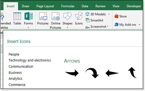
Inserting Icons
Excel 2019 offers a series of royalty-free icons that can be added to your worksheet. To start, use the Icons button on the Insert tab of the ribbon. Provided you are connected to the Internet, a series of icons in 26 categories will appear in the Insert Icons dialog box, as shown in Figure 26.21.
To insert an icon, select the icon and then press Insert.
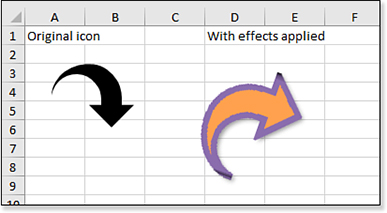
Once inserted into your worksheet, you can use the Graphic Tools Format tab of the ribbon to change the color, outline, and bevel. Handles on the icon allow you to change the size and rotations. Figure 26.22 shows some of the effects.
Examining 3D Models
There are a large number of 3D Models available on the Internet. Excel 2019 can import files saved with any of these extensions: *.fbx, .obj, .3mf, .ply, .stl, and .glb. A large number of 3D Model files are available from NASA. Point your favorite search engine at NASA 3D Models to find them.
Select, Insert, 3D Models, From File, and select a model. Initially, the model appears in the worksheet as shown in Figure 26.23.

With the object selected, click the 3D Rotation icon and drag it in any direction.
Dragging right and left will rotate sideways.
Dragging up and down will rotate vertically.
Dragging diagonally will rotate diagonally.
If you drag far enough, the object will rotate so you can see the back side of the object.