IDA’s external graphing capability utilizes third-party graphing applications to display IDA-generated graph files. For Windows versions prior to 6.1, IDA ships with a bundled graphing application named wingraph32.^[55] For IDA 6.0, non-Windows versions of IDA are configured to use the dotty^[56] graph viewer by default. Beginning with IDA 6.1, all versions of IDA ship with and are configured to use the qwingraph^[57] graph viewer, which is a cross-platform Qt port of wingraph32. While the dotty configuration options remain visible for Linux users, they are commented out by default. The graph viewer used by IDA may be configured by editing the GRAPH_VISUALIZER variable in <IDADIR>/cfg/ida.cfg.

Whenever an external-style graph is requested, the source for the graph is generated and saved to a temporary file; then the designated third-party graph viewer is launched to display the graph. IDA supports two graph specification languages, Graph Description Language^[58] (GDL) and the DOT^[59] language utilized by the graphviz^[60] project. The graph specification language used by IDA may be configured by editing the GRAPH_FORMAT variable in <IDADIR>/cfg/ida.cfg. Legal values for this variable are DOT and GDL. You must ensure that the language you specify here is compatible with the viewer you have specified in GRAPH_VISUALIZER.

Five types of graphs may be generated from the View ▸ Graphs submenu. Available external mode graphs include the following:

For two of these, the flowchart and the call graph, IDA is capable of generating and saving GDL (not DOT) files for use independently of IDA. These options may be found on the File ▸ Produce file submenu. Saving the specification file for other types of graphs may be possible if your configured graph viewer allows you to save the currently displayed graph. A number of limitations exist when dealing with any external graph. First and foremost is the fact that external graphs are not interactive. Manipulation of displayed external graphs is limited by the capabilities of your chosen external graph viewer (often only zooming and panning).

External Flowcharts

With the cursor positioned within a function, View ▸ Graphs ▸ Flow Chart (hotkey F12) generates and displays an external flowchart. The flowchart display is the external graph that most closely resembles IDA’s integrated graph-based disassembly view. These are not the flowcharts you may have been taught during an introductory programming class. Instead, these graphs might better be named “control flow graphs,” as they group a function’s instructions into basic blocks and use edges to indicate flow from one block to another.

Figure 9-6 shows a portion of the flowchart of a relatively simple function. As you can see, external flowcharts offer very little in the way of address information, which can make it difficult to correlate the flowchart view to its corresponding disassembly listing.

Figure 9-6. External flowchart graph

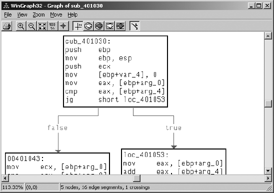
Flowchart graphs are derived by following the ordinary and jump flows for each instruction in a function, beginning with the entry point to the function.

External Call Graphs

A function call graph is useful for gaining a quick understanding of the hierarchy of function calls made within a program. Call graphs are generated by creating a graph node for each function and then connecting function nodes based on the existence of a call cross-reference from one function to another. The process of generating a call graph for a single function can be viewed as a recursive descent through all of the functions that are called from the initial function. In many cases, it is sufficient to stop descending the call tree once a library function is reached, as it is easier to learn how the library function operates by reading documentation associated with the library rather than by attempting to reverse engineer the compiled version of the function. In fact, in the case of a dynamically linked binary it is not possible to descend into library functions, since the code for such functions is not present within the dynamically linked binary. Statically linked binaries present a different challenge when generating graphs. Since statically linked binaries contain all of the code for the libraries that have been linked to the program, related function call graphs can become extremely large.

In order to discuss function call graphs, we make use of the following trivial program that does nothing other than create a simple hierarchy of function calls:

#include <stdio.h>

void depth_2_1() {
   printf("inside depth_2_1
");
}

void depth_2_2() {
   fprintf(stderr, "inside depth_2_2
");
}

void depth_1() {
   depth_2_1();
   depth_2_2();
   printf("inside depth_1
");
}

int main() {
   depth_1();
}

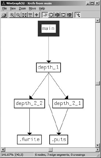
After compiling a dynamically linked binary using GNU gcc, we can ask IDA to generate a function call graph using View ▸ Graphs ▸ Function Calls, which should yield a graph similar to that shown in Figure 9-7. In this instance we have truncated the left side of the graph somewhat in order to offer a bit more detail. The call graph associated with the main function can be seen within the circled area in the figure.

Figure 9-7. External function call graph

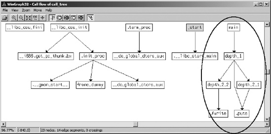
Alert readers may notice that the compiler has substituted calls to puts and fwrite for printf and fprintf, respectively, as they are more efficient when printing static strings. Note that IDA utilizes different colors to represent different types of nodes in the graph, though the colors are not configurable in any way.^[62]

Given the straightforward nature of the previous program listing, why does the graph appear to be twice as crowded as it should be? The answer is that the compiler, as virtually all compilers do, has inserted wrapper code responsible for library initialization and termination as well as for configuring parameters properly prior to transferring control to the main function.

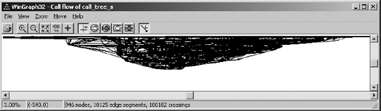
Attempting to graph a statically linked version of the same program results in the nasty mess shown in Figure 9-8.

The graph in Figure 9-8 demonstrate a behavior of external graphs in general, namely that they are always scaled initially to display the entire graph, which can result in very cluttered displays. For this particular graph, the status bar at the bottom of the WinGraph32 window indicates that there are 946 nodes and 10,125 edges that happen to cross over one another in 100,182 locations. Other than demonstrating the complexity of statically linked binaries, this graph is all but unusable. No amount of zooming and panning will simplify the graph, and beyond that, there is no way to easily locate a specific function such as main other than by reading the label on each node. By the time you have zoomed in enough to be able to read the labels associated with each node, only a few dozen nodes will fit within the display.

Figure 9-8. Function call graph in a statically linked binary

External Cross-Reference Graphs

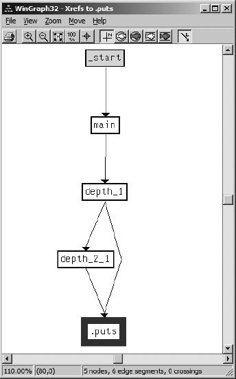
Two types of cross-reference graphs can be generated for global symbols (functions or global variables): cross-references to a symbol (View ▸ Graphs ▸ Xrefs To) and cross-references from a symbol (View ▸ Graphs ▸ Xrefs From). To generate an Xrefs To graph, a recursive ascent is performed by backtracking all cross-references to the selected symbol until a symbol to which no other symbols refer is reached. When analyzing a binary, you can use an Xrefs To graph to answer the question, “What sequence of calls must be made to reach this function?” Figure 9-9 shows the use of an Xrefs To graph to display the paths that can be followed to reach the puts function.

Figure 9-9. Xrefs To graph

Similarly, Xrefs To graphs can assist you in visualizing all of the locations that reference a global variable and the chain of function calls required to reach those locations. Cross-reference graphs are the only graphs capable of incorporating data cross-reference information.

In order to create an Xrefs From graph, a recursive descent is performed by following cross-references from the selected symbol. If the symbol is a function name, only call references from the function are followed, so data references to global variables do not show up in the graph. If the symbol is an initialized global pointer variable (meaning that it actually points to something), then the corresponding data offset cross-reference is followed. When you graph cross-references from a function, the effective behavior is a function call graph rooted at the selected function, as shown in Figure 9-10.

Unfortunately, the same cluttered graph problems exist when graphing functions with a complex call graph.

Figure 9-10. Xrefs From graph

Custom Cross-Reference Graphs

Custom cross-reference graphs, called User xref charts in IDA, provide the maximum flexibility in generating cross-reference graphs to suit your needs. In addition to combining cross-references to a symbol and cross-references from a symbol into a single graph, custom cross-reference graphs allow you to specify a maximum recursion depth and the types of symbols that should be included or excluded from the resulting graph.

View ▸ Graphs ▸ User Xrefs Chart opens the graph customization dialog shown in Figure 9-11. Each global symbol that occurs within the specified address range appears as a node within the resulting graph, which is constructed according to the options specified in the dialog. In the most common case, generating cross-references from a single symbol, the start and end addresses are identical. If the start and end addresses differ, then the resulting graph is generated for all nonlocal symbols that occur within the specified range. In the extreme case where the start address is the lowest address in the database and the end address is the highest address in the database, the resulting graph degenerates to the function call graph for the entire binary.

Figure 9-11. User cross-reference graph dialog

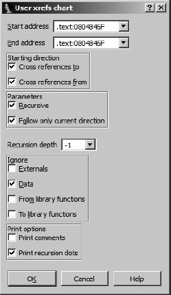
The options that are selected in Figure 9-11 represent the default options for all custom cross-reference graphs. Following is a description of the purpose of each set of options:

Starting direction

Options allow you to decide whether to search for cross-references from the selected symbol, to the selected symbol, or both. If all other options are left at their default settings, restricting the starting direction to Cross references to results in an Xrefs To–style graph, while restricting direction to Cross references from generates an Xrefs From–style graph.

Parameters

The Recursive option enables recursive descent (Xrefs From) or ascent (Xrefs To) from the selected symbols. Follow only current direction forces any recursion to occur in only one direction. In other words, if this option is selected, and node B is discovered to be reachable from node A, the recursive descent into B adds additional nodes that can be reached only from node B. Newly discovered nodes that refer to node B will not be added to the graph. If you choose to deselect Follow only current direction, then when both starting directions are selected, each new node added to the graph is recursed in both the to and from directions.

Recursion depth

This option sets the maximum recursion depth and is useful for limiting the size of generated graphs. A setting of −1 causes recursion to proceed as deep as possible and generates the largest possible graphs.

Ignore

These options dictate what types of nodes will be excluded from the generated graph. This is another means of restricting the size of the resulting graph. In particular, ignoring cross-references from library functions can lead to drastic simplifications of graphs in statically linked binaries. The trick is to make sure that IDA recognizes as many library functions as possible. Library code recognition is the subject of Chapter 12.

Print options

These options control two aspects of graph formatting. Print comments causes any function comments to be included in a function’s graph node. If Print recursion dots is selected and recursion would continue beyond the specified recursion limit, a node containing an ellipsis is displayed to indicate that further recursion is possible.

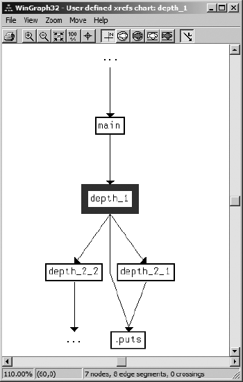
Figure 9-12 shows a custom cross-reference graph generated for function depth_1 in our example program using default options and a recursion depth of 1.

Figure 9-12. User xref graph for function depth_1

User-generated cross-reference graphs are the most powerful external-mode graphing capability available in IDA. External flowcharts have largely been superseded by IDA’s integrated graph-based disassembly view, and the remaining external graph types are simply canned versions of user-generated cross-reference graphs.

With version 5.0, IDA introduced a long-awaited interactive, graph-based disassembly view that was tightly integrated into IDA. As mentioned previously, the integrated graphing mode provides an alternative interface to the standard text-style disassembly listing. While in graph mode, disassembled functions are displayed as control flow graphs similar to external-style flowchart graphs. Because a function-oriented control flow graph is used, only one function at a time can be displayed while in graph mode, and graph mode cannot be used for instructions that lie outside any function. For cases in which you wish to view several functions at once, or when you need to view instructions that are not part of a function, you must revert to the text-oriented disassembly listing.

We detailed basic manipulation of the graph view in Chapter 5, but we reiterate a few points here. Switching between text view and graph view is accomplished by pressing the spacebar or right-clicking anywhere in the disassembly window and selecting either Text View or Graph View as appropriate. The easiest way to pan around the graph is to click the background of the graph view and drag the graph in the appropriate direction. For large graphs, you may find it easier to pan using the Graph Overview window instead. The Graph Overview window always displays a dashed rectangle around the portion of the graph currently being displayed in the disassembly window. At any time, you can click and drag the dashed rectangle to reposition the graph display. Because the graph overview window displays a miniature version of the entire graph, using it for panning eliminates the need to constantly release the mouse button and reposition the mouse as required when panning across large graphs in the disassembly window.

There are no significant differences between manipulating a disassembly in graph mode and manipulating a disassembly in text mode. Double-click navigation continues to work as you would expect it to, as does the navigation history list. Any time you navigate to a location that does not lie within a function (such as a global variable), the display will automatically switch to text mode. Graph mode will automatically be restored once you navigate back to a function. Access to stack variables is identical to that of text mode, with the summary stack view being displayed in the root basic block of the displayed function. Detailed stack frame views are accessed by double-clicking any stack variable, just as in text mode. All options for formatting instruction operands in text mode remain available and are accessed in the same manner in graph mode.

The primary user interface change related to graph mode deals with the handing of individual graph nodes. Figure 9-13 shows a simple graph node and its related title bar button controls.

Figure 9-13. Typical expanded graph view node

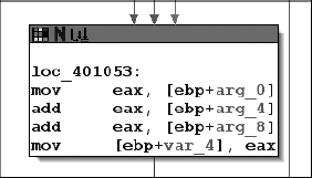
From left to right, the three buttons on the node’s title bar allow you to change the background color of the node, assign or change the name of the node, and access the list of cross-references to the node. Coloring nodes is a useful way to remind yourself that you have already analyzed a node or to simply make it stand out from others, perhaps because it contains code of particular interest. Once you assign a node a color, the color is also used as the background color for the corresponding instructions in text mode. To easily remove any coloring, right-click the node’s title bar and select Set node color to default.

The middle button on the title bar in Figure 9-13 is used to assign a name to the address of the first instruction of the node’s basic block. Since basic blocks are often the target of jump instructions, many nodes may already have a dummy name assigned as the result of being targeted by a jump cross-reference. However, it is possible for a basic block to begin without having a name assigned. Consider the following lines of code:

.text:00401041               jg      short loc_401053
.text:00401043               mov     ecx, [ebp+arg_0]

The instruction at has two potential successors, loc_401053 and the instruction at . Because it has two successors, must terminate a basic block, which results in becoming the first instruction in a new basic block, even though it is not targeted explicitly by a jump and thus has no dummy name assigned.

The rightmost button in Figure 9-13 is used to access the list of cross-references that target the node. Since cross-reference comments are not displayed by default in graph mode, this is the easiest way to access and navigate to any location that references the node. Unlike the cross-reference lists we have discussed previously, the generated node cross-reference list also contains an entry for the ordinary flow into the node (designated by type ^). This is required because it is not always obvious in graph view which node is the linear predecessor of a given node. If you wish to view normal cross-reference comments in graph mode, access the Cross-References tab under Options ▸ General and set the Number of displayed xrefs option to something other than zero.

Nodes within a graph may be grouped either by themselves or with other nodes in order to reduce some of the clutter in a graph. To group multiple nodes, ctrl-click the title bar of each node to be grouped and then right-click the title bar of any selected node and select Group nodes. You will be prompted to enter some text (defaults to the first instruction in the group) to be displayed in the collapsed node. Figure 9-14 shows the result of grouping the node in Figure 9-13 and changing the node text to collapsed node demo.

Figure 9-14. Typical collapsed (grouped) graph view node

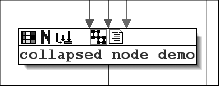
Note that two additional buttons are now present in the title bar. In left-to-right order, these buttons allow you to uncollapse (expand) the grouped node and edit the node text. Uncollapsing a node merely expands the nodes within a group to their original form; it does not change the fact that the node or nodes now belong to a group. When a group is uncollapsed, the two new buttons just mentioned are removed and replaced with a single Collapse Group button. An expanded group can easily be collapsed again using the Collapse Group button or by right-clicking the title bar of any node in the group and selecting Hide Group. To completely remove a grouping applied to one or more nodes, you must right-click the title bar of the collapsed node or one of the participating uncollapsed nodes and select Ungroup Nodes. This action has the side effect of expanding the group if it was collapsed at the time.