
At this point, you’ve run through the techniques in the preceding chapters (especially Chapters 6, 7, and 8) and determined that the GPU, not the CPU or another resource, is your bottleneck. Fantastic! Optimizing the GPU can be a lot of fun.
As always, you will want to measure carefully after each change you make. Even if the GPU were initially the bottleneck, it might not be after a few optimizations. Be sure to keep your mental picture of your game’s performance up to date by regularly measuring where time is going.
Optimizing GPU performance is fun because it varies so much. The general rule is always the same—draw only what is needed. But the details shift. Each generation of graphics hardware changes the performance picture. Each generation of games has more required of it by its audience.
You can break GPUs into three broad tiers. Fixed function GPUs have no or limited programmability. They can only apply textures or do other shading or transformation calculations in certain fixed ways, which is what gives them their name. You most often find these cards in cheap consumer hardware—low-end game consoles, portable devices, and budget systems. The Nintendo DS, the pre-3Gs iPhones and iPod Touches, and the Wii all fall into this category.
We consider programmable GPUs to be shader GPUs. These are so named because they can run user shader programs to control various parts of the rendering process. Programs are run at the vertex, pixel, and geometry level. Nearly every card made by any manufacturer in the past decade supports shaders in some way. Consoles like the Xbox 360 and PS3, and nearly all desktop PCs, have cards that fall into this category.
Finally, there are unified GPUs. These are pure execution resources running user code. They do not enforce a specific paradigm for rendering. Shader Model 4.0 cards fall into this categorycrecent vintage cards from ATI and NVIDIA, for the most part. At this tier, the capabilities of the hardware require special consideration, which we highlight in Chapter 16, “GPGPU.”
Each tier of GPU can perform the operations of the preceding tier. You can exactly emulate a fixed-function GPU with a shader GPU, and a shader GPU can be exactly emulated with a unified GPU. But each tier also adds useful functionality and allows you to operate under a less constrained set of assumptions when it comes to optimizing.
The decision as to which tier of hardware to target will be determined by your game’s target audience. If you are developing a Wii game, your decision is made for you. If you are developing a PC game, you will need to do some research to see what level of graphics hardware your audience has. Targeting the latest and greatest is a lot of fun from a development perspective, but it can be unfortunate for sales when only a few users are able to run your game well!
Sometimes, it is worthwhile to optimize for income. And it is always nicer to develop on lower-end hardware and find at the end that you have done all the optimization you need, instead of developing on high-end hardware and finding you have major performance issues to resolve at the end of your project.
The rendering pipeline in 3D cards has evolved over the years. Figure 9.1 shows the last few generations of the Direct3D pipeline, from DirectX 8 through 10. As you can see, there has been a heavy trend from fixed-purpose hardware to having nearly every part of the pipeline be programmable.
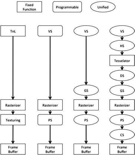
Figure 9.1. Evolution of graphics pipelines. From left to right, DirectX 7, DirectX 8.1, DirectX 9, and DirectX 10/11. Not shown, the shift in fundamental capabilities of the hardware from fixed to shader-based to fully programmable hardware.
Chapter 4, “Hardware Fundamentals” goes into more detail, but, in general, work flows from the top to the bottom of the pipeline. Each point of added programmability (shown as ellipitical circles in Figure 9.1) makes it easier to build complex visual effects. These points also provide opportunities to tune performance.
How do you tell if you’re GPU bound? To summarize quickly, if you see that you’re spending a lot of time in API calls, especially draw calls or calls to swap/present the framebuffer, it’s likely that the CPU is waiting for the GPU to finish drawing.
Tools like PIX, PerfView, Intel’s GPA, GPU Perf Studio, and others (discussed in Chapter 3, “The Tools”) will analyze the GPU’s performance statistics. If you see that you have zero GPU idle time and high CPU idle time, it’s another clear indicator that you are GPU limited. These tools will give you a clear idea of what is taking up the most time on the GPU.
If you know you are GPU bound, the next step is to look at where the time is going, and to do that you have to look at what is going on in the source of rendering a frame.
A frame can be visualized as a series of events taking place on the GPU. Each event, determined by your API calls, is data being copied or processed in some way. Keep in mind that the GPU maintains a queue of commands to execute, so the actual results of an API call might not be calculated until several previous frames’ worth of rendering are completed.
In the case of PIX, you get a direct visualization of the event execution on the timeline view. In the absence of a PIX-like tool, you can infer the behavior with careful timing. There are also ways to force synchronization (discussed in Chapter 8).
All this is to say that your goal as a GPU optimizer is to identify the events that are taking up the most execution resources and then optimize them. It’s the Pareto Principle at work again—20% of GPU activity tends to take up 80% of time and space. Of course, sometimes you will find a situation where the workload is even. In that case, it will be a slow grind to reduce drawing and find enough small wins to get the performance win you need.
Are you limited by geometry or pixels? You can break the pipeline into a front and back end as an aid to optimization. The front end deals with setting up triangles and other geometry for drawing, while the back end handles processing pixels, running shaders, and blending the results into the framebuffer.
How do you test to see which half is the bottleneck? It’s easy—vary the workload for one half and see if overall performance varies. In the case of the GPU, the simple test is to reduce the render target size. You can do this most simply by setting the scissor rectangle to be just a few pixels in size. All geometry will still have to be processed by the front end, but the vast majority of the work for the back end can be quickly rejected.
// Make a one pixel scissor rect.
RECT testRect = {0, 0, 1, 1};

// Set the scissor rect.
pD3DDevice->SetScissorRect(testRect);
pD3DDevice->SetRenderState(D3DRS_SCISSORTESTENABLE, true);
Notice that we chose a scissor rectangle more than zero pixels in size. Graphics cards do have to produce correct output, but if they can save processing time, they will. So it is reasonable for them to optimize the zero-size scissor rectangle by simply ignoring all draw operations while the scissor is relevant. This is why it is essential to measure on a variety of cards because not all of them use the same tricks for gaining performance.
Warnings aside, it should be pretty clear if the front end (geometry) or back end (pixels) is your bottleneck by the performance difference from this quick test. If there is a performance gain, then you know that per-pixel calculations are the bottleneck.
You will notice the subsequent sections here are organized based on whether they are related to the front end or the back end. We will start from the back, where pixels are actually drawn, and work our way to the front, where draw commands cause triangles to be processed. Because the later stages of the pipeline tend to involve the bulk of the work and are also easier to detect and optimize, we’ll start with them.
Fill-rate is a broad term used to refer to the rate at which pixels are processed. For instance, a GPU might advertise a fill-rate of 1,000MP/sec. This means it can draw one hundred million pixels per second. Of course, this is more useful if you can convert it to be per frame. Say you want your game to run at 60Hz. Dividing 1,000MP/sec by 60Hz gives a performance budget on this theoretical card of 17MP/frame.
Another consideration is overdraw. Overdraw occurs when a given location on the screen is drawn to more than once. You can express overdraw as a coefficient. If you draw to every pixel on the screen once, you have the ideal overdraw of one. If you draw to every pixel on the screen 10 times, you have an unfortunate overdraw of 10. Since most applications draw different content to different parts of the screen, overdraw is rarely a whole number.
Many graphics performance tools include a mode to visualize overdraw. It’s also easy to add it on your own—draw everything with alpha blending on and a flat transparent color. Leave the Z test, culling, and all other settings the same. If you choose, say, translucent red, then you will see bright red where there is lots of overdraw and dim red or black where there is little overdraw.
Finally, you should consider your target resolution. You can express your target resolution in megapixels. If you are targeting 1,920 × 1,080, then you are displaying approximately 2.0 megapixels every frame. This is useful because, combined with average overdraw, target frame rate, and fill-rate budget, you have a relationship that governs your performance.
GPU fill rate / Frame rate = Overdraw * resolution
You can plug in your values and solve to see how much overdraw you can budget per frame.
1000MP/sec / 60Hz = Overdraw * 2MP
17MP/frame = Overdraw * 2MP
Overdraw = 8.5
Now you know that, from a fill-rate perspective, you cannot afford more than 8.5x overdraw. That sounds pretty good! But you shall see as we move through the next few sections that even a generous budget can get used up very quickly.
The first factor that directly impacts fill-rate is the format of your render target. If you are drawing in 16-bit color, fewer bytes have to be written for every pixel. If you are writing each channel as a 32-bit floating-point value, a lot more data must be written. On PC hardware, the best-supported format is R8G8B8A8, and it’s a good place to start. Extremely narrow formats can actually cause a performance loss, because they require extra work to write. Sometimes, you need wider formats for some rendering tasks. If you suspect that the bottleneck is reading/writing the framebuffer, vary the format. If you see a performance change, then you know that the format is a bottleneck.
We’ll look at the implications of varying pixel formats later in the section, “Texture Sampling.”
The first factor that can consume fill-rate is blending. Enabling alpha blending causes the hardware to read back the existing value from the framebuffer, calculate the blended value based on render settings and the result of any active textures/shaders, and write it back out.
In our test results shown in Figure 9.2, we found that drawing alpha-blended pixels consumes approximately 10% more fill-rate on our NVIDIA GTX 260.
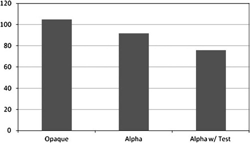
Figure 9.2. Comparison of drawing a fixed number of opaque, alpha tested, and alpha blended pixels. A small test texture was active while drawing.
Enabling alpha testing gained even more performance, although that will vary depending on your art.
There are several strategies you can use to reduce the cost of translucent objects. The first is to draw them as opaque. This gets you the fastest path.
The next is to use alpha testing if you need transparency not translucency. (Transparency means you can see through parts of an object, like a chain link fence, while translucency means light filters through the object, like a stained glass window.) Alpha testing is also good because it is compatible with the Z-buffer, so you don’t have to do extra sorting to make sure alpha-tested geometry is drawn at the right time.
Finally, you can go to approximations. There are a variety of order-independent, depth-sorted translucency techniques available (all with limitations, all with a high performance cost). Sometimes, dithering is an option. Distant translucent objects could be drawn as opaque to save fill-rate, too.
You can tell if blending is your bottleneck by a simple test—disable alpha blending and draw opaque! If you see a performance gain, your bottleneck is alpha blending.
The performance implications of pixel shaders are so big that we had to devote Chapter 10, “Shaders,” to fully consider them. On most fixed-function hardware available to PCs, the relative cost of none, flat, and Gouraud shading is minimal. (If you are targeting a more limited GPU, like on a mobile device, you may want to run some quick tests.)
Textures can cost a lot of fill-rate! Each texture sampled to draw a pixel requires resources to fetch data from memory, sample it, and combine into a final drawn pixel. The main axes we will consider here are texture format, filter mode, and texture count. In the case of programmable GPUs, the “combine” step will be discussed in Chapter 10, while in the case of fixed-function GPUs, the combine step is implemented in hardware and is usually overshadowed by the cost of the texture fetches.
Figure 9.3 shows the performance effects of various texture formats. You can see that 16- and 32-bit textures are the cheapest, while DXT1 gives pretty good performance at nearly 80% memory savings. Performance doesn’t quite scale linearly with bit depth, but that’s a good approximation.
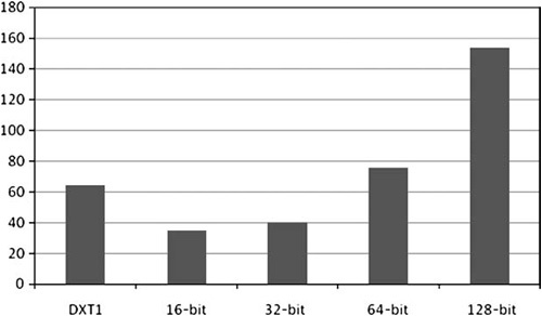
Figure 9.3. Comparison of fill-rate when drawing geometry using textures with different sized pixels.
Filtering is a little harder to analyze because it can be affected by the orientation of the rendered surfaces. To combat this, in our measurements of various texture-sampling modes (shown in Figure 9.4), we adjusted our test geometry to get a good distribution of samples and sizes. The same random seed was used for each run of the test to get comparable results.
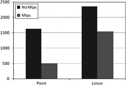
Figure 9.4. Comparison of various sampling modes with mipmapping on and off. The test geometry was drawn at random orientations to ensure realistic results.
As you can see, enabling mipmapping is a major performance win. Turning on linear sampling almost exactly triples the cost per pixel, but it is a major quality win.
Figure 9.5 shows the performance drop from sampling more textures. As you can see, it gets worse and eventually plateaus.
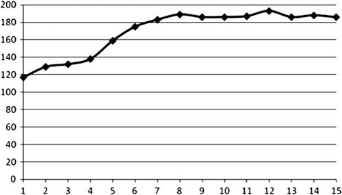
Figure 9.5. Comparison of performance (Y-axis, in milliseconds) with varying number of active textures (X-axis). Bilinear filtering and mipmapping were enabled for all textures.
Bear in mind that with shaders you can do dependent or conditional texture samples, which can dramatically alter the performance picture. We’ll discuss this wrinkle in the next chapter.
If you suspect that texture sampling is a bottleneck, the best test is to replace all your textures with a single small 4x4 test texture and disable samplers where possible. Because such a small texture easily fits in the GPU’s texture cache, you should see a significant speedup. If so, you know that texture sampling is your bottleneck.
The Z-buffer is a major tool for increasing rendering performance. Conceptually, it is simple. If the fragment to be drawn to a given pixel is farther than what is already drawn there, reject it. GPU manufacturers have since introduced two major enhancements.
First, you have hierarchical Z, which is where the GPU maintains a version of the Z-buffer data that can be hierarchically sampled. This allows the GPU to reject (or accept) whole blocks of pixels at once, rather than testing each individually. API and vendor documentation go into the specifics of how this is implemented for each GPU, most importantly covering what, if any, settings or actions will cause hierarchical Z to be disabled. All GPUs on the PC market today support it, so we will not be doing any tests targeting it specifically.
Often, the hierarchical structure degrades as drawing occurs, so it is necessary to reset it. This is done when a Z-clear is issued. The usual Z-clear at the start of rendering is sufficient.
Second, you have fast Z writes, which are enabled by disabling color writes. When this mode is active, the GPU skips most shading calculations, enabling it to draw significantly faster. Why is this useful? If you draw the major occluders in your scene with fast-Z before drawing the scene normally, it gives you an opportunity to reject many pixels before they are even shaded. Depth tests occur at the same place in the pipeline as alpha tests, giving significant savings when the depth tests can reject pixels.
The stencil buffer can also be used for culling (among other operations). Stencil tests occur at the same stage in the pipeline as depth and alpha tests, allowing for very fast pixel rejection.
Clearing the framebuffer is an important operation. If the Z-buffer and stencil buffer aren’t reset every frame, rendering will not proceed correctly. Depending on the scene, failing to clear the color channels will result in objectionable artifacts. Clearing is another commonly accelerated operation, since setting a block of memory to a fixed value is an embarrassingly parallel operation.
Generally, you should only issue clears at the start of rendering to a render target. A common mistake is to issue clears multiple times, either on purpose or due to bugs in code. This can quickly devour fill-rate. Generally, applications are not bound by the performance of clears, but the best policy is to make sure that you clear no more than is strictly necessary for correct results.
The front end is where geometry and draw commands are converted into pixels to be drawn. Performance problems occur here less often, but they still happen. Don’t forget to run the stencil test at the beginning of the chapter to determine if the front or back end is your bottleneck!
If the front end is a bottleneck, there are three main potential causes: vertex transformation, vertex fetching, and caching, or tessellation. Most of the time, scenes are not vertex-bound because there are just so many more pixels to render. But it can happen.
In general, fewer vertices are better. You should never be drawing triangles at a density of greater than one per pixel. For a 1,080p screen, this suggests that more than 2MM triangles onscreen at a time is more than you need. Of course, your source art is liable to have an extremely high polygon count, so you should be using LOD to reduce workload at runtime.
Vertex transformation is the process of converting vertex and index data fetched from memory into screen coordinates that can be passed to the back end for rasterization. This is the compute part of the vertex performance picture, where vertex shaders are executed. On fixed-function cards, where vertex processing isn’t programmable, there are usually lighting, texture coordinate generation, and skinning capabilities.
You can test whether vertex transformation is a bottleneck very simply: simplify the transformation work the GPU must do. Remove lighting calculations, replace texture coordinate generation with something simple (but not too simple, as simply writing out a fixed coordinate will favor the texture cache and alter performance elsewhere), and disable skinning. If there’s a performance gain, you’ll know that vertex transformation is a bottleneck.
On fixed-function hardware, usually all you can do is disable features to gain performance. On old or particularly low-end programmable hardware, be aware that the vertex programs may be run on the CPU. This can shift your system-level loads rather unexpectedly, as work that should be on the GPU is done on the CPU. We will discuss optimizing vertex shaders in Chapter 10.
Index data is processed in order, and vertex data is fetched based on the indices you specify. As you will remember from Chapter 6, “CPU Bound: Memory,” memory is slow. The GPU can fight this to a certain degree. Indexed vertices are not hard to pre-fetch. But there is only limited cache space, and once the cache is full, pre-fetching can’t hide latency.
As you know, geometry is submitted to the GPU in the form of primitives. The most common types are triangle lists and triangle strips. Strips have the benefit of having a smaller memory footprint, but the bigger issue by far (see Figure 9.6) is how many cache misses are encountered while the vertices are being fetched. Maximizing vertex reuse is crucial, and most 3D rendering libraries include code for optimizing vertex order. Of particular interest is the D3DXOptimizeVertices call from D3DX and “Linear-speed Vertex Cache Optimization” by Tom Forsyth, 2006, at http://home.comcast.net/~tom_forsyth/papers/fast_vert_cache_opt.html.
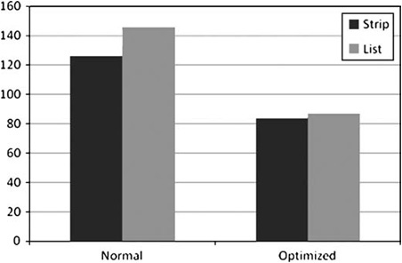
Figure 9.6. Performance of various primitive types representing the Stanford Bunny, drawn in cache-friendly order and in random order.
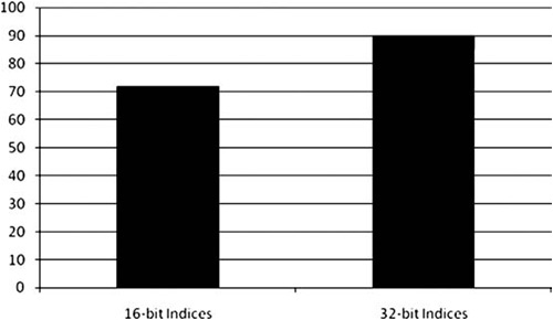
There are two other major considerations for performance in this area. First, index format. The two options here are 16-bit and 32-bit indices. See Figure 9.7 for a comparison of performance with these options. Note that not all cards properly support 32-bit indices.
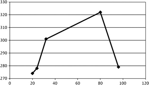
The other consideration is vertex format, specifically vertex size. By reducing the total dataset that must be processed to render a mesh, you can gain some performance. Figure 9.8 shows the variation for different vertex sizes. As you can see, there is a cost for large and odd vertex sizes.
The final major performance bottleneck is tessellation. More recent GPUs with DXll tessellation capabilities can alter, delete, and emit new geometry via geometry shaders. We will discuss this capability in more detail in the next chapter.
Many older GPUs feature different tessellation capabilities, but unless you are targeting a specific card, they are not flexible or powerful enough to warrant spending the time on custom art and one-shot code. It’s better to spend the effort to make your game run well on many GPUs and systems.
In addition to the main pipeline discussed previously, there are several other wrinkles that can affect your performance.
Multisample antialiasing is a technique for supersampling an image. Originally, it was done by rendering the scene at a high resolution and downsampling. Now more exotic techniques are used, with varying performance implications. The specific details are interesting, but beyond the scope of this book. What is relevant is that MSAA can significantly affect fill-rate.
Lighting and shadows can be a major performance problem in all but the simplest scenes. They do not have a simple fix. Lighting can require a lot of data to get right. Shadows can stress the entire rendering pipeline, from CPU to vertex processing to pixel processing, because they often require drawing the whole scene from multiple viewpoints every frame.
A survey of all the rendering techniques for lighting and shadowing is well beyond our scope, and it would probably be obsolete as soon as it was printed. Instead, we’d like to give some general guidelines.
Remember that lighting quality is a matter of perception. Great art can make up for minimal or nonexistent lighting. Humans have an intuitive understanding of lighting, but what looks good and serves the purposes of gameplay doesn’t necessarily have anything to do with the physical reality of the game space. (Illustrative Rendering in Team Fortress 2 by Mitchell, Francke, and Eng has an interesting discussion of the trade-offs here in section 5.)
In general, consistency is the most important attribute for lighting to have. It should not have discontinuities or obvious seams. The human eye is very good at noticing that, say, a whole object becomes dark when it cross through a doorway, or that different parts of a character are lit differently with seams between them. People will accept very simple lighting calculations if they do not have objectionable artifacts.
Take advantage of the limited scenarios your game offers to cheat. You can design your levels and other assets so that performance drains and problematic cases never occur. It will be a temptation to implement a total lighting solution that deals with every case well. Resist this. Determine the situations your game has to support and make sure they work well. Ignore the rest.
Ultimately, lighting calculations are done for every pixel on the screen. They might be interpolated based on values calculated per vertex. They might be calculated based on some combined textures or with multiple passes that are composited. They might be done in a pixel shader. In the end, multiple light and shadow terms are combined with material properties to give a final color for each pixel on the screen.
This brings us to the first performance problem brought by lighting: It can require you to break up your scene and your draw calls. If you are using the built-in fixed-function lighting, a vertex shader or a pixel shader, each object will require a different set of constants (or a call to set the lighting properties). For small mobile meshes, like those that make up characters, vehicles, and items, a single set of constants can hold all the information needed to light that object. But for larger objects, like a terrain or a castle, different parts of the object will need to be lit differently. Imagine a castle lit by a sunrise with dozens of torches burning in its hallways.
It is generally cost prohibitive to render every light’s effect on every object in the scene, so most engines maintain a lookup structure to find the N closest lights. This way, if only four lights can be efficiently considered for a material, the four most important lights can be found and supplied for rendering.
For larger objects, it can make sense to calculate lighting as a second pass. If the lit area is significantly smaller than the whole object, redrawing just the affected geometry can be a big savings. In some cases, just the triangles affected can be streamed to the GPU dynamically. For more complex meshes, this can be cost-prohibitive, so an alternative is to group geometry into smaller chunks that can be redrawn without requiring per-triangle calculations.
While lights are important, shadows are the interaction between lights and objects, and they bring a lot of realism to any scene. Shadowing is generally implemented by rendering depth or other information to a texture and then sampling that texture in the shaders of affected objects. This consumes fill-rate when rendering, as well as introducing the overhead of rendering to and updating the texture(s) that define the shadows. As alluded to earlier, this is essentially a second (or third or fourth or fifth) scene render.
The nice thing about shadows is that they do not require the fidelity of a full scene render. Post-processing effects are not needed. Color doesn’t matter—just the distance to the closest occluder. A lot of the overhead of sorting, of setting material properties, and so on can be avoided.
In the end, lighting systems are built on the primitives we have discussed already in this chapter. There is a lot to say about lighting and shadowing in terms of getting good quality and performance, but once you know how to fit them into your optimization framework, it becomes a matter of research and tuning to get the solution your game needs. The optimization process is the same as always. Find a benchmark, measure it, detect the problem, solve, check, and repeat.
The biggest game changer, as far as performance goes, is deferred rendering. The traditional model is forward rendering, where objects are composited into the framebuffer as rendering proceeds. If you were to take a snapshot of the framebuffer after each render call, it would look pretty much like the final frame (with fewer objects visible).
In deferred rendering, normals, material types, object IDs, lighting information, and other parameters are written to one or more render targets. At the end of this process, the rich buffer of data produced is processed to produce the final image displayed to the user. This significantly simplifies rendering, because even scenes with many lights and shadows can be processed in a uniform way. The main problem a forward renderer faces, with regard to lighting, is getting multiple shadows and lights to interact in a consistent way.
But creating the data for the final deferred pass is not cheap. It requires a very wide render target format or multiple render targets. A lot of fill-rate is consumed when moving all this data around, and the shader for the final pass can be costly. In general, though, deferred rendering acts to flatten performance—it is not great, but it doesn’t get a lot worse as scene complexity grows.
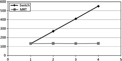
We’ve already discussed rendering to wide render targets. It is also possible to render to multiple render targets at the same time. This is referred to as MRT. It can be a useful technique for deferred shading, for shadow calculations, and for optimizing certain rendering algorithms. However, it does not come without cost.
MRT is not available on all hardware, but when it is available, it’s a clear win, as Figure 9.9 shows.
A GPU is a complex and multifaceted beast, but with care, research, and discipline, it is capable of great performance. From API to silicon, GPUs are designed to render graphics at incredible speed. In this chapter, we covered the GPU pipeline from the performance perspective, and shared tests, performance guidelines, and recommendations for getting the best performance from each stage. Don’t forget to run the performance test harness on your own graphics hardware. The best way to get great performance is to measure, and the test harness is the easiest way to do that.