Chapter 6

Analysis of Variance From Two or More Populations

In prior chapters, we explored the analysis of numerical data from one and two populations. This chapter expands our discussion of population means to accommodate the simultaneous analysis of multiple populations. With the increased complexity of multiple populations, we may find common attributes that cross the populations of interest and affect the variable we want to study. In such circumstances, appropriate design of the experiment generating the data to be analyzed becomes essential. More than other chapters, then, this chapter focuses on the experimental design leading to data collection for analysis. We will continue our discussion of means and variances of numerical data, but we will develop analytic tools to compare multiple population means with a new capability to identify and account for the effect of a confounding variable. We will continue to use sample statistics, standard errors, and acceptable levels of significance in calculating test statistics. All F-tests in analysis of variance are conducted as one-tailed tests.

The Design of Experiments

In our review of analysis of variance, shortened to the acronym ANOVA, we will consider three basic experimental designs: single factor, two-factor without replication, and two-factor with replication. The analyses differ not in the kind of data gathered but the way in which the data are gathered.

In single factor ANOVA, also referred to as one-way ANOVA, a single variable is measured for random samples taken from multiple populations. The data are grouped as samples from each of the populations of interest. The number of groups in the data represent the number of populations sampled, which is also the number of levels of the factor being analyzed. If, for example, we are interested in the lengths of time to complete an athletic event for participating athletes from five different age groups, then each athlete’s time to completion is the variable being measured and the measurements will be sorted into one of the five different age groups. Age is the factor being analyzed. This ANOVA has five levels of the single factor, age. The analysis of completion times will seek to determine whether the average completion time differs across the five different age groups. Because we want to see completion times change as a function of age groups, in this example, age is an independent variable and time to completion is the dependent variable. The analysis can accommodate different numbers of sampled elements at each of the factor levels—that is, we would not have to sample the same number of athletes in each age group.

In two-factor ANOVA without replication, a single numerical variable generates data from multiple populations. Elements are sampled from each of the populations of interest. But a second classification cuts across the multiple populations, creating a grid that guides our selection of population elements in a specific way. We randomly sample a single element from each of the multiple populations that represents each of the levels of the second classification. So, for example, if we are interested in the lengths of time to complete an athletic event and we have five different age groups, but we suspect an athlete’s weight may affect the recorded completion times, we can use ANOVA to separate the effects of age groups and weight classes on the dependent variable, time to completion. Let us assume for this example that four different weight categories are identified. In two-factor ANOVA without replication, we would sample a total of 20 athletes, one athlete at each of the four weight categories within each of the five age groups. Again we would record each athlete’s time to completion as the variable being measured, and the measurements would be carefully placed in each cell of the data grid. The analysis of completion times can determine whether the average completion time differs across the five different age groups, as well as whether average completion time differs across the four different weight classes. In this example, both age and weight are independent variables and completion time is the dependent variable. The number of elements sampled is restricted to the product of the number of levels for the two independent variables, age and weight.

Two-factor ANOVA with replication is designed similarly to two-factor ANOVA without replication, with the exception that we have multiple elements for each combination of categories for the independent variables. For the problems we will deal with in this chapter, the number of elements in each cell must be the same, so the total elements sampled must be some multiple times the number of cells in the data grid. If, to continue our example, we have five age groups and four weight classes, for two-factor ANOVA with replication we would then plan to sample 40 athletes or 60 athletes or 80 athletes, and so on, where the number of replications is the number of athletes sampled for each cell of the age-weight class data grid. With two-factor ANOVA with replication, we can test for the interactive effects of age and weight classes. Such results might show that older and heavier athletes perform differently than younger and lighter athletes. If interaction effects are not significant, the analyst can then test for the individual main effects of age and weight.

Single-Factor ANOVA: The Completely Randomized Design

Single-factor ANOVA is the simplest of the experimental designs used in ANOVA. While it can be used to analyze differences in two population means, its strength is best shown in testing differences among means from three or more populations. In one light, elements sampled for single-factor ANOVA can be seen as members of a single, broad population, who are randomly assigned to different treatment groups and, following treatment, are then measured on some dimension to determine the effect of each treatment. For example, the tensile strength of rope woven three different ways from the same fiber source can be compared to determine if the weaving introduces different average strength to one rope than to the others. In another light, single-factor ANOVA can be viewed as a tool to analyze a single variable as it exists within distinctly different populations. For example, the tensile strength of ropes woven the same way from different fiber sources can be compared to determine if the average strength of one rope woven from one fiber differs from the average strength of ropes woven from other fibers. Both applications of single-factor ANOVA are appropriate. To conduct single-factor ANOVA, the dependent variable must be approximately normally distributed in each of the populations sampled and the variances of the dependent variable must be approximately equal in each of the populations.

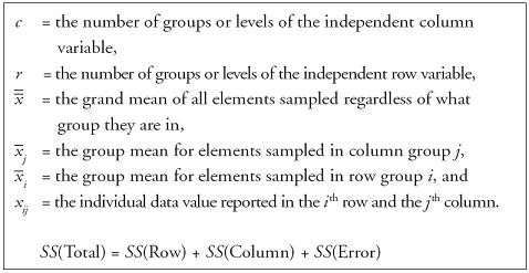
The single-factor analysis of variance is based on the sum of squared differences between individual data values and their group and grand means. The total variation is formed by the sum of the squared differences between all elements sampled and the grand mean of the sampled elements regardless of what group or level they are assigned to or represent. The total variation is parsed into between-groups variation (variation that is explained by an element’s membership in a particular group) and within-groups variation (variation that is unexplained by an element’s group membership). Mathematically, we can summarize these relationships with the following equations:

Variation must be converted to variance before we can begin to discuss conducting tests of hypotheses, because it is the ratio of variances, as we saw in the prior chapter, that leads to the F-test. To form variance, the sum of squares (SS) is divided by its degrees of freedom, forming the column headed by MS in Table 6.1.

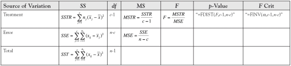
The F-statistic is formed by the ratio of the between-groups variance divided by the within-groups variance. A large between-groups variance and a small within-groups variance lead to a large F-statistic. The larger the F-statistic is, the smaller its p-Value and the more likely we are to reject the null hypothesis, which is our objective in structuring a hypothesis test in the first place. The degrees of freedom for the F-statistic are given by the degrees of freedom on the numerator and the denominator—that is, (c − 1) for the numerator and (n − c) for the denominator. Although the equations to perform the analysis by hand are given in Table 6.1, Excel’s Data Analysis toolkit has a menu choice that will automate the analysis of raw data, which we use here.

Example 6.1.

An experimental project was run in mature navel orange orchards in Central California managed by three different companies. The number of fancy grade fruit produced by trees in each of their orchards were sampled and recorded for the last year. Assume the number of fruit is approximately normally distributed and the sampled trees were randomly and independently selected. Use the Excel printout shown in Table 6.2 to determine whether there is evidence at the 5% level of significance of a difference in the average number of fruit produced in the three orchards.

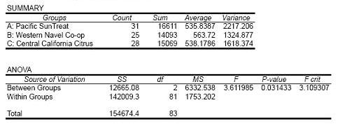
Answer

H₀: μ_A = μ_B = μ_C

H₁: At least one of the means differs from the rest.

Decision Rule: For α = 0.05 with numerator df = 2 and denominator df = 81, we will reject the null hypothesis if the calculated test statistic falls above F = 3.109.

Test Statistic:

Observed Significance Level:

p-value = 0.031

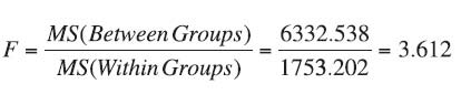
Conclusion: Since the test statistic of F = 3.612 falls above the critical bound of F = 3.109, we reject H₀ with at least 95% confidence. Likewise, since the p-value of 0.031 is less than the desired α of 0.05, we reject H₀. There is enough evidence to conclude that at least one of the orchards achieved a different average production than the other two orchards.

Two-Factor ANOVA Without Replication: The Randomized Block Design With One Observation in Each Cell

Two-factor ANOVA without replication allows us to add a second dimension to the comparison of means across treatment groups accomplished in single-factor ANOVA. This analysis assumes the two dimensions are independent of one another. Like single-factor ANOVA, two-factor ANOVA without replication is an additive model in that the total sum of squares is parsed between explained variation and unexplained variation. By adding a second factor to the experimental design, two-factor ANOVA without replication allows us to account for additional fluctuation in the dependent variable that we suspect is associated with a second variable but that is not fully explained by the primary variable. In adding a second factor to the analysis, we further reduce the unexplained within-group variation, SS(Error), which in turn, which leads to a smaller mean square error (MSE) in the denominator to the F-statistic, and a stronger test result.

While single-factor ANOVA allows groups of varying sample sizes, the addition of a second variable in two-factor ANOVA creates a data grid that confines and prescribes the sampling design the researcher using two-factor ANOVA without replication must follow. Specifically, if there are r levels in the row variable and c levels in the column variable, then the data grid across which the sampled elements are recorded is r by c with n = (r • c) total number of cells. This new sampling design requires one sampled element for each cell.

Example 6.2.

To examine the heights in inches of three different varieties of pepper plants, an experimental project was run on four plots with different soil types. Assume plant heights are approximately normally distributed. Use the Excel printout shown in Table 6.3 to determine whether there is evidence at the 5% level of significance of a difference in the average heights of plants by soil plot and by seed variety.

Answer: Testing Across Soil Plots

We can test for differences in average plant height across soil plots, where soil plots represents the row variable, as follows:

H₀: μ₁ = μ₂ = μ₃ = μ₄

H₁: At least one of the means differs from the rest.

Decision Rule: For α = 0.05 with numerator df = 3 and denominator df = 6, we will reject the null hypothesis if the calculated test statistic falls above F = 4.757.

Test Statistic:

Observed Significance Level:

p-value = 0.0266

Conclusion: Since the test statistic of F = 6.412 falls above the critical bound of F = 4.757, we reject H₀ with at least 95% confidence. Likewise, since the p-value of 0.0266 is less than the desired α of 0.05, we reject H₀. There is enough evidence to conclude that at least one of the soil plots produces different average plant height from the other soil plots.

Answer: Testing Across Seed Varieties

We can test for differences in average plant height across seed varieties, where seed varieties represents the column variable, as follows:

H₀: μ_A = μ_B = μ_C

H₁: At least one of the means differs from the rest.

Decision Rule: For α = 0.05 with numerator df = 2 and denominator df = 6, we will reject the null hypothesis if the calculated test statistic falls above F = 5.143.

Test Statistic:

Observed Significance Level:

p-value = 0.0171

Conclusion: Since the test statistic of F = 8.637 falls above the critical bound of F = 5.143, we reject H₀ with at least 95% confidence. Likewise, since the p-value of 0.0171 is less than the desired α of 0.05, we reject H₀. There is enough evidence to conclude that at least one of the seed varieties produces different average plant height from the other seed varieties.

Two-Factor ANOVA With Replication: The Factorial Design With m Observations in Every Cell

Two-factor ANOVA with replication reports the analysis of data captured in a grid with r levels of the row variable, c levels of the column variable, and m data values in every cell of the data grid. The number of replications in the r by c design is m. Two-factor ANOVA with replication allows us to investigate whether the row and column variables are independent of one another or whether the variables interact to affect the values recorded for the dependent variable. This is the comparative benefit of using a factorial design associated with two-factor ANOVA with replication. If interaction effects are not significant, individual row and column effects can be interpreted as they were in the prior section. If an interaction effect exists in the data, the level that occurs on one dimension has some differential effect on the dependent variable depending on the level occurring on the other dimension. For example, if the age and weight class of an athlete have an interactive effect on the time to completion of an athletic event, then a younger and lighter athlete might perform differently than other younger athletes and other lighter athletes.

If interaction effects are significant in the data, individual effects of the row and column variables are difficult to interpret. In the presence of interaction among the row and column variables, we cannot say that the means for the row levels or the means for the column levels are significantly different because the row means change depending on the column level or, alternatively, the column means change depending on the row level. The variables are, in fact, not independent of one another. By removing that variation that is due to interaction, the remaining unexplained variation is reduced, leading to a smaller mean square error and potentially larger, more significant, F-ratios for the main effects of the row and column variables than might otherwise be warranted. Finding significant interaction in a set of data complicates our analysis of them, and the researcher should take caution to avoid erroneous interpretations of main effects.

Example 6.3.

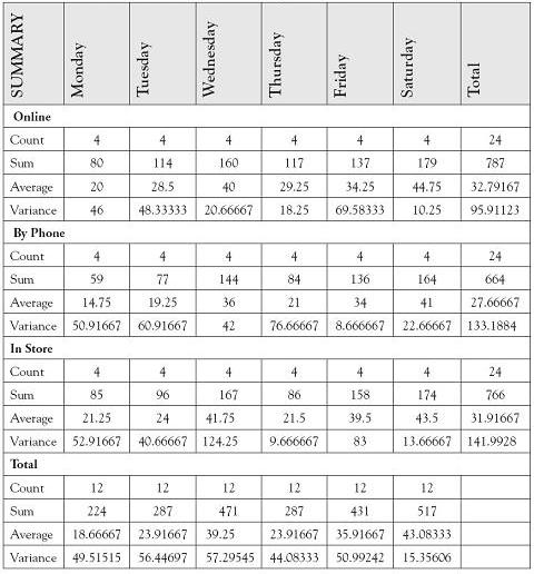
A company’s marketing executive ran an experiment on product sales sites. Specifically, she collected product sales completed online, by phone, and in store sites for 4 weeks by weekdays. Since the store and phone sites were closed on Sundays, she limited the data to Mondays through Saturdays. Data are shown in Table 6.4.

Use a 5% level of significance to analyze mean differences. Specifically test for whether there is any significant interaction between day of week and sales site. If interaction is not significant, test for main effects of day of week and sales site.

Answer: Testing for an Interaction Effect

We can test for an interaction between the two variables day of week and sales site as follows:

H₀: There is no interaction between day of week and sales site.

H₁: There is an interaction between day of week and sales site.

Decision Rule: For α = 0.05 with numerator df = 10 and denominator df = 54, we will reject the null hypothesis if the calculated test statistic falls above F = 2.011.

Test Statistic:

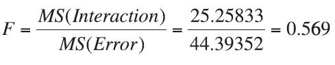
Observed Significance Level:

p-value = 0.8318

Conclusion: Since the test statistic of F = 0.569 falls below the critical bound of F = 2.011, we do not reject H₀ with at least 95% confidence. Likewise, since the p-value of 0.8318 is greater than the desired α of 0.05, we do not reject H₀. There is not enough evidence to conclude that there is any significant interaction between day of week and sales site. Based on this conclusion, we can proceed to test for difference by sales site and by day of week.

Answer: Testing Across Sales Sites

We can test for differences among average sales by sales sites, where sales sites represents the row variable, as follows:

H₀: μ_Online = μ_Phone = μ_Store

H₁: At least one of the average sales differs by sales site.

Decision Rule: For α = 0.05 with numerator df = 2 and denominator df = 54 we will reject the null hypothesis if the calculated test statistic falls above F = 3.168.

Test Statistic:

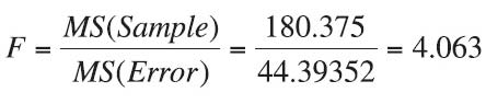
Observed Significance Level:

p-value = 0.0227

Conclusion: Since the test statistic of F = 4.063 falls above the critical bound of F = 3.168, we reject H₀ with at least 95% confidence. Likewise, since the p-value of 0.0227 is less than the desired α of 0.05, we reject H₀. There is enough evidence to conclude that there is a difference in the average sales made at different sales sites.

Answer: Testing Across Days of the Week

We can test for differences among average sales by days of the week, where days of the week represents the column variable, as follows:

H₀: μ_M = μ_Tu = μ_W = μ_Th = μ_F = μ_S

H₁: At least one of the average sales differs by day of week.

Decision Rule: For α = 0.05 with numerator df = 5 and denominator df = 54, we will reject the null hypothesis if the calculated test statistic falls above F = 2.386.

Test Statistic:

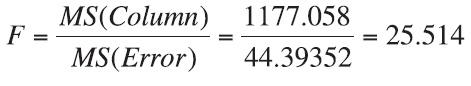
Observed Significance Level:

p-value = 2E-13, which means 2 × 10⁻¹³, which is very small.

Conclusion: Since the test statistic of F = 25.514 falls well above the critical bound of F = 2.386, we reject H₀ with at least 95% confidence. Likewise, since the p-value of 2 × 10⁻¹³ is much smaller than the desired α of 0.05, we reject H₀. There is enough evidence to conclude that there is a difference in the average sales made at different days of the week.

We have shown in Example 6.3. that at least one of the average sales differs by sales site as well as by day of week. There are statistical procedures that can be used to determine which of the pairs of means are significantly different. For example, we can follow up the ANOVA with a test of whether Monday sales differ significantly from Tuesday sales. Care must be taken to properly consider the statistical significance of several pair-wise mean differences taken from the same data set. We will not address the advanced procedures here, but the motivated researcher can access further information using the Tukey simultaneous confidence interval for the difference of two means. The citation can be researched in almost any standard statistical textbook and on the Internet.