Chapter 4

Using Proof by Contradiction to Draw Conclusions

Uncertainty is a fact of life. We often have good evidence to support our claims or our beliefs. We seldom have irrefutable evidence of the important ones. In statistics, the process by which we gather information and link it as evidence to our claims or beliefs is called scientific, or hypothesis, testing. It is, at its heart, a proof by contradiction. A proof by contradiction goes something like this:

1. Assume as true the opposite of what you are testing for.
2. Envision what data should look like if that opposite were, in fact, true.
3. Gather data relating to the claims, and compare the vision for the data and the actual data gathered.
4. Draw a conclusion from the comparison and interpret its meaning in terms of the research question.

What researchers hope to draw is a negative conclusion. That is, researchers want to show that the data they gathered are so unlikely to come from a world in which the assumption made in step 1 is true that they must conclude the assumption is not true, is contradicted. Some new terminology will help us develop this chain of logic. The null hypothesis is a formal statement about the population that is consistent with the assumption in step 1. Often the null hypothesis is a statement about a population parameter that characterizes what has been typical of the population in the past, that nothing will change in that population, that the status quo will continue. It is denoted by H₀. The alternative hypothesis is the challenge posed by research that, if shown true, will cause a change to the status quo. It is sometimes called the research hypothesis since it is the reason the research is undertaken in the first place. It is denoted by H₁ and is stated in a manner that is the opposite of the statement in the null hypothesis, H₀.

The Hypotheses: Making a Claim

Forming hypotheses is the first step of any analytic project. Because it contains the reason for the research, the alternative hypothesis is often easier to form first. Let’s investigate several research scenarios.

Scenario 1: Product containers are filled with 6 ounces (170 grams) of salted nuts. If the containers are overfilled, the product does not ship well and does not hold its shelf life. If the containers are underfilled, the company risks a fine from consumer advocates. Samples of 50 containers are randomly selected and individual product weights are taken and recorded. If the containers are either over or under filled, the quality control officer will halt the production line and schedule maintenance to service the machines.

In Scenario 1, the quality control officer will continue production as usual as long as the average container weight is 6 ounces. The officer will alter the current production flow if there is evidence that the average container weight is not 6 ounces. So the best null and alternative hypotheses are the following:

H₀: μ = 6 H₁: μ ≠ 6

This is a nondirectional, two-tailed test.

Scenario 2: The air quality index (AQI) is a system used by local and national agencies to report on how clean or polluted the air is. The AQI ranges from 0, which indicates no risk of pollution, to 500, which carries a hazardous warning for the entire population. An AQI in the range of 101 to 150 means the air is unhealthy for sensitive groups, who may experience some health effects as a result of air pollution. If the AQI is 150 or less, the general public is not likely to be affected. If the AQI is above 150, everyone may begin to experience health effects. If the AQI is above 150, a media announcement is activated to warn local residents that air quality is unhealthy.

In Scenario 2, the general public is not at risk if the AQI is 150 or less. The general public is at risk if the AQI is above 150. To determine whether the air quality is good and the general public is at little or no health risk as a result, or whether air quality is sufficiently bad to cause some health risk to the general public, the best null and alternative hypotheses are the following:

H₀: μ ≤ 150 H₁: μ > 150

This is a directional, upper-tailed test.

Scenario 3: Regional management for a large chain of home construction and improvement stores has indicated that at least 60% of all items on their store shelves must have individual prices marked on the items. Individual store managers are being notified that inspectors will be surveying shelved inventories. Managers of stores that do not meet the guideline will be cited.

In Scenario 3, managers will not be cited if 60% or more of their shelved inventories are marked with the item price. Managers will be cited if less than 60% of their shelved inventories are marked with the item price. So the best null and alternative hypotheses are the following:

H₀: p ≥ 0.60 H₁: p < 0.60

This is a directional, lower-tailed test.

In all three scenarios, the entire number line is covered by the null and alternative hypotheses. This is true, in fact, of all pairs of null and alternative hypotheses. This is also true whether the hypothesis test is two-tailed, as in Scenario 1, or one-tailed, as in Scenarios 2 and 3. A second important point arises from investigating these three scenarios: in all three scenarios, the equal sign is included in the null hypothesis. This too is true of all pairs of null and alternative hypotheses. It means that there must be more than enough evidence to conclude the alternative hypothesis is true to warrant changing the status quo.

A final but important note about forming hypotheses: while the contexts given in this book are predefined as appropriate for a one- or two-tailed test, the researcher should be careful about structuring a one-tailed hypothesis test. Two-tailed tests are generally most appropriate except where reason, historic record, or known effects persuade the researcher to structure and perform a one-tailed test.

The Decision Rule: Setting Error Tolerance

With hypotheses in place, the researcher next must play out the null hypothesis. The null hypothesis is assumed to be true. The researcher must ask: if the null hypothesis were true, what should we expect to see? In the formal hypothesis test, this step creates a decision rule. For example, if, in Scenario 1, the mean is equal to 6 ounces, then sample means will likely fall no further than some specified number of units of standard error away from the center, 6 ounces. If, in Scenario 2, the mean AQI is less than or equal to 150, then air samples will generate means that are no more than a specific number of units of standard error above 150. If, in Scenario 3, the proportion is greater than or equal to 0.60, then sample proportions taken from that population will fall no less than some specified number of units of standard error below 0.60.

While a well-adjusted production line may occasionally produce a sample of 50 containers whose average weight is well above or below the intended mean of 6 ounces, it is not very probable to occur. After all, when the machines truly are well adjusted, that means they are achieving an average fill of 6 ounces per container. In evaluating a sample mean that occurs outside the expected window of production on either side of the mean of 6 ounces, making a decision to stop the line and schedule maintenance to adjust the machines requires the quality control manager to accept a certain level of risk that the decision is in error. That risk is called a Type I error and is denoted by α. Alpha (α) is the probability that a true null hypothesis is incorrectly rejected. In the research scenario, the sample mean is all the decision maker has, however, to then infer whether the sample could have come from a population located at μ. A decision maker cannot be 100% certain that the sample whose mean falls in an outer tail isn’t just an odd sample that really did come from a sampling distribution whose mean is located at μ. So the decision maker must accept a Type I error of probability α in order to set a limit on how unusual a sample can be before they decide that the sample is just too different to believe it came from a population that was actually centered at μ. The critical bound defines that limit. Since 100α% is the error a researcher is willing to accept, 100(1 − α)% is the level of confidence the decision maker has in deciding the hypothesis test results.

In a one-tailed hypothesis test, α appears in one tail of the distribution. In fact, α appears in the tail that the alternative hypothesis designates. The Type I error, α, is the amount of area left in the tail beyond the critical z or t bound, or the amount of area in the rejection region, as shown in Figures 4.1 and 4.2.

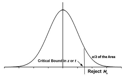
H₀: A population parameter ≤ A specific value H₁: A population parameter > A specific value

H₀: A population parameter ≥ A specific value H₁: A population parameter < A specific value

In a two-tailed hypothesis test, the Type I error, α, is split between the upper and lower tail. So the amount of area in any one tail of the distribution is α/2, as shown in Figure 4.3. The amount of error in deciding the hypothesis test is still α, and the amount of confidence the researcher has in the results continues to be 100(1 − α)%.

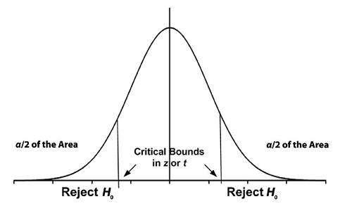
H₀: A population parameter = A specific value
H₁: A population parameter ≠ A specific value

The Test Statistic

Evaluating the sample data is perhaps the easiest step of conducting a hypothesis test. At this stage, the researcher should collect the data and calculate the sample statistics (for example, , s, or ). Using the values of the sample statistics and hypothesized value of the population parameter, the test statistic (for example, z or t) can be calculated.

Compared to the first step of framing appropriate null and alternative hypotheses, and the second step of determining an appropriate Type I error and decision rule, the third step of computing the sample statistic is relatively straightforward. Gathering good data may be time consuming, but the design for gathering and analyzing the data should be completed in the first two steps of the research project. As we will see later in this chapter, we will use one of several general equations in computing a statistic that we will then compare to the acceptable window around the population measure.

Good research practice should complete the statement of hypotheses and the decision rule before collecting the data and calculating the statistics. Even if the data were technically collected in advance of the study, prior analysis of the data should not be used to structure the hypotheses or set the error tolerance.

Drawing a Conclusion

The fourth step in the process of hypothesis testing is drawing a conclusion and tying it specifically to the problem environment. The sense of the conclusion we draw is not a statement of immutable truth, nor is it something we can say with absolute certainty. The conclusion is a statement based on probability. It is probably true. There is a small chance that the decision is in error. Reaching a conclusion is perhaps best characterized as an assertion warranted by the evidence we have brought to bear on the null hypothesis. As such, when we state the conclusion, we should reflect the sample statistic, the decision rule, the conclusion, and the amount of confidence we have in making the statement. A second statement is useful in reflecting back on the problem environment to indicate what the conclusion means in the problem’s context.

In summary, then, a formal hypothesis test should include the following:

1. The null hypothesis and the alternative hypothesis
2. The decision rule, which includes both a statement of the Type I error the decision maker is willing to accept in order to make a decision, as well as the acceptable window around the population measure
3. The value of the sample statistic
4. The conclusion and its interpretation

One final note about hypothesis testing: a proof by contradiction requires that the null hypothesis is assumed to be true. The conclusion can refute that assumption, or not. That is, the researcher can conclude that the test statistic is so unusual, the sample cannot have come from a population centered at μ. Or the researcher can conclude that the test statistic is not unusual enough to reject the null hypothesis. What the researcher cannot conclude is that the null hypothesis must be true. Why not? Because the null hypothesis was assumed to be true to begin with, a researcher cannot then conclude that the null hypothesis must be true. That would constitute circular logic: you cannot prove true what you assumed was true in the first place. To avoid this fundamental error in logic, we adopt the convention of concluding either that we have sufficient evidence to reject the null hypothesis or we do not have sufficient evidence to allow us to reject the null hypothesis. We cannot conclude that we accept the null hypothesis.

The p-Value: The Observed Significance Level

The observed significance level, known as the p-value, is based on two elements of the hypothesis test: the value of the test statistic and the hypotheses being tested. While the level of significance of the test, α, is a value the decision maker sets at the beginning of the research, the observed significance level, the p-value, is determined by the results of the sample data. The p-value is the probability that a sample statistic based on another random sample selected from the same population is at least as extreme as the calculated sample statistic. Because it is based on the sample statistic, the p-value is called the observed significance level of the test statistic.

The p-value is a measure of how different the sample is from the hypothesized population. A p-value can be calculated for any sample statistic as it relates to its theoretical distribution. We will discuss p-values for test statistics related to the t-distribution, the z-distribution, the F-distribution, and the χ²-distribution. The p-value is particularly useful because it cuts across theoretical distributions. It is often referenced in publications following a research conclusion, shown in parentheses to communicate the strength of the evidence supporting the research conclusion.

In a one-tailed hypothesis test, the p-value is the amount of area beyond the test statistic into the tail of the rejection region. To find it on the z-distribution, we simply look the test statistic up on the Cumulative Standard Normal Table. If the p-value is smaller than α, then the test statistic itself falls beyond the critical bound of the rejection region. When that happens, the null hypothesis is rejected. If the p-value is larger than α, then the test statistic falls between the population parameter and the boundary of the rejection region. When that happens, the null hypothesis cannot be rejected.

In a two-tailed hypothesis test, sample data are just as likely to be positive as negative. So the amount of area beyond the test statistic into the tail of the distribution is only half of the p-value. To get the full p-value, the area beyond the test statistic has to be doubled. Comparisons of the p-value and α are then conducted as indicated in a one-tailed hypothesis test.

Testing Hypotheses Involving μ When σ Is Known

Human behavior and performance typically vary widely and vary differently over different populations. When dealing with human performance, it is usually the case that variance on their measures is not known. Some exceptions occur when significant historical data exist from which accurate evaluations of variance can be derived. In contrast, many mechanical processes are designed so that mean performance and variance on mean performance can be controlled within machine tolerances.

In instances where σ is known and the underlying population is normally distributed, the sampling distribution of the mean will be normally distributed regardless of the sample size taken. In instances where σ is known but the underlying population is not normally distributed, sampling distributions of the mean are approximately normally distributed when the sample size is sufficiently large. Knowing that the sampling distribution of the mean is normally or approximately normally distributed allows us to standardize the sample mean with reference to the standard normal distribution using the following equation:

Example 4.1.

A commercial processing plant fills containers with 6 ounces (170 grams) of salted nuts. Machinery on the production line is set to maintain a variance of 0.008 ounces. If the containers are either over or under filled, the quality control officer will halt the production line and schedule maintenance to service the machines. Samples of 50 containers are randomly selected and individual product weights are taken and recorded. The last sample of 50 containers produced a mean of 5.9775 ounces. Should the line be shut down for maintenance? Use a 5% level of significance.

Answer

H₀: μ = 6
Average container weight is 6 ounces. The machinery does not need additional service.

H₁: μ ≠ 6
Average container weight is not 6 ounces. The machinery does need additional service.

Decision Rule: Since this is a two-tailed test, the alpha level of 0.05 is split in half, half allocated to the upper tail and half to the lower tail of the rejection region. See Figure 4.3. For α = 0.05, then, we identify the critical bound associated with an 0.9750 on the z-table, because the central area of 0.95 and the lower tail of 0.025 are combined. We will reject the null hypothesis if the calculated test statistic falls above z = 1.96 or below z = −1.96.

Test Statistic:

Observed Significance Level: For a z-score of −1.78, the probability is 0.0375 of getting a z-score of −1.78 or more negative. Since this is a two-tailed test, the test statistic could just as likely be +1.78 or greater. So the area below the z of −1.78 is only half of the total area to be included. The full p-value is then twice the area captured below the test statistic of z = −1.78.

p-value = 2 • (0.0375) = 0.0750

Conclusion: Since the test statistic of z = −1.78 falls between the critical bounds of ±1.96, we do not reject H₀ with at least 95% confidence. Likewise, since the p-value of 0.0750 is greater than the desired α of 0.05, we do not reject H₀. There is not enough evidence to conclude the machinery needs additional service. The line should not be shut down for maintenance.

Connection Between the Hypothesis Test and the Confidence Interval

In Chapter 3, we introduced the notion and calculations for the confidence interval. We looked at confidence intervals on the mean and on the proportion. Although the goal of a confidence interval is different from the goal of a hypothesis test, there is still a very real connection between them. Put simply, for the two-tailed hypothesis test, if the value we test in the null hypothesis falls between the upper and lower bounds of the confidence interval, the conclusion of the hypothesis test will not reject H₀. And, for the two-tailed hypothesis test, if the value we test in the null hypothesis falls outside of the confidence interval bounds, the conclusion of the hypothesis test will reject H₀. For a one-tailed hypothesis test, we should compare the value in the null hypothesis to the confidence interval bounds calculated for twice the value of the significance level used for the hypothesis test, so that 100α% of the area is in both the rejection region of the hypothesis test and one tail of the confidence interval. To demonstrate the connection, we return to Example 4.1 and compute the 95% confidence interval around the sample mean of 5.9775:

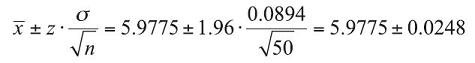
The lower bound on the mean container weight is 5.9527 ounces, and the upper bound is 6.0023 ounces. Since the hypothesized mean of 6 ounces is contained in the 95% confidence interval around the sample mean, we fail to reject the comparable hypothesis that the true mean could be different from 6 ounces based on this sample with the comparable 95% confidence level.

Testing Hypotheses Involving μ When σ Is Unknown

When the population variance, σ, is not known, the sample size must be sufficiently large to satisfy requirements of the Central Limit Theorem for us to use the t-distribution as an approximation of the sampling distribution.

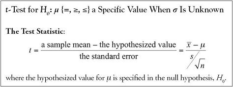
We need to discuss the process of identifying the appropriate t-coefficient to use as the critical bound in hypothesis tests using the t as the test statistic. To identify the critical bound in t, we enter the t-table with two pieces of information from the problem we wish to solve: (1) the degrees of freedom, and (2) the amount of area in the tail of the t-distribution. In the case of an upper-tail t-test with, for example, 7 degrees of freedom and α = 0.05, we would identify t = 1.895 as the appropriate critical bound for the rejection region. In the case of a lower-tail t-test with 7 degrees of freedom and α = 0.05, we would identify t = −1.895 as the appropriate critical bound for the rejection region.

In the case of a two-tailed t-test with 7 degrees of freedom and α = 0.05, we would identify t = ±2.365 as the appropriate critical bounds for the rejection region.

Example 4.2.

According to the Food Marketing Institute, the average sales per customer transaction for supermarkets in the United States was $27.61 in 2008. Suppose management of a regionally owned supermarket believed their average sales per customer transaction is higher than the value for the nation as a whole. They took a random sample of 60 customer transactions and found their mean to be $31.24 with a standard deviation of $8.15. Is there sufficient evidence to conclude with 99% confidence that their average customer transaction is higher than the average for the nation as a whole?

Answer

H₀: μ ≤ $27.61
Average sales per customer transaction is less than or equal to $27.61.

H₁: μ > $27.61
Average sales per customer transaction is greater than $27.61.

Because the population value σ is not known, we use the sample value s to approximate it. So we use the t-distribution, not the z-distribution.

Decision Rule: Since this is a one-tailed test, the alpha level of 0.01 is entirely in the upper tail of the rejection region. See Figure 4.1. For α = 0.01 with 59 degrees of freedom, we will reject the null hypothesis if the calculated test statistic falls above t = 2.391.

Test Statistic:

Observed Significance Level: To find an exact p-value for a t statistic, we use Excel’s imbedded function =tdist(3.45,59,1), which yields the answer: p-value = 0.000521.

Conclusion: Since the test statistic of t = 3.45 falls above the critical bound of 2.391, we reject H₀ with at least 99% confidence. Likewise, since the p-value of 0.0005 is less than the desired α of 0.01, we reject H₀. There is enough evidence to conclude that the average sales per customer transaction for this regionally owned supermarket is higher than the average for the nation as a whole.

Testing Hypotheses Involving p When n Is Sufficiently Large

• Who does the grocery shopping more often for a typical household? The male or the female head of household?
• What proportion of vehicles involved in traffic crashes are light trucks?
• What percent of plumbing parts shipped to retailers and distributors last year were domestically made?
• Is your favorite candidate leading by a comfortable margin two weeks before the election?
• Does the percent of defective products produced increase during the night shifts?

Sometimes what we want to know cannot be measured. In answering the sample of questions above, we would not measure things but count them. We would count male and female heads of households who report more often doing the grocery shopping; the total number of traffic crashes and the number that involved light trucks; the total number of plumbing parts made last year and the number that were domestically made, etc. Theoretically, the appropriate distribution to reference is a discrete distribution because the underlying variables are discrete counts. It has been shown that if the sample sizes are sufficiently large, the z-distribution is a very good approximation of the sampling distribution of the proportion that is created by a ratio of the counts generated. To successfully convert a discrete distribution to the z-distribution, both n • p and n • (1 − p) must be greater than or equal to 5.

Example 4.3.

According to the American Institute of Architects in their second quarter 2010 survey, 31.3% of residential architects identified an in-home office as the most popular special feature of new households. Suppose a random sample of 100 homebuilders reported that 28% of new homebuyers were specifically looking for a residence with an in-home office. Are homebuilders reporting results that differ significantly from the information provided by the American Institute of Architects? Use a 90% level of confidence.

Answer

H₀: p = 0.313
The proportion of homebuyers who are specifically looking for a residence with an in-home office is the same as the information provided by the American Institute of Architects.

H₁: p ≠ 0.313
The proportion of homebuyers who are specifically looking for a residence with an in-home office differs from the information provided by the American Institute of Architects.

Decision Rule: For α = 0.10, we will reject the null hypothesis if the calculated test statistic falls above z = 1.645 or below z = − 1.645.

Test Statistic:

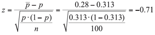
Observed Significance Level: p-value = 2•(0.2389) = 0.4778

Conclusion: Since the test statistic of z = −0.71 falls between the critical bounds of ±1.645, we do not reject H₀ with at least 90% confidence. Likewise, since the p-value of 0.4778 is greater than the desired α of 0.10, we do not reject H₀. There is not enough evidence to conclude that the proportion of homebuyers differ significantly from the information provided by the American Institute of Architects (http://www.aia.org/practicing/AIAB085952).