Chapter 8

Analyzing Bivariate Data

We often find it telling to collect data that track two quantitative variables simultaneously. We may want to look at changes in one variable as it changes with or perhaps even influences values of a second variable. How loosely or tightly connected two variables are can be quantified using the methods introduced in this chapter. One method, called regression analysis, explores whether we can improve our estimate of one variable by knowing the value of the other variable for an element of the population being studied. A unique benefit of regression analysis arises from the regression model itself: We can use the regression model to predict values of interest from information that is already known. By using recent information on automobile loan rates, for example, we can anticipate the rate we might qualify for as we decide what car to buy. Knowing how the rates have changed over time in recent weeks or even days, we can better predict the rate we can lock in at the time of our purchase. By knowing sales of a product in recent days, managers can better estimate how deep an inventory to maintain and how often to refresh their order to meet but not greatly exceed consumer demand for the product. Or, by knowing the annual return on a stock, a trader might be able to predict its future market value. Values of interest are sometimes dependent on several inputs. The market value of a stock, for example, may be influenced by a number of factors. We will limit regression analysis in this chapter to the relationship between a single independent variable, x, and its dependent variable, y.

Scatterplots

Sometimes a relationship between two numerical random variables becomes apparent by collecting a random sample of measurements of both variables and looking at an x-y scatterplot of the data. Seldom do we see a relationship between two variables so tightly connected that the scatterplot maps to a straight line. More likely, the data points are somewhat dispersed, or scattered, around the grid. A cloud of data points that generally rises from left to right provides evidence of a positive or direct relationship between the two variables, whereas a cloud of points that falls from left to right provides evidence of a negative or inverse relationship between x, the independent variable, and y, the dependent variable. A cloud of points that appears as a smattering of points with no direction to them provides evidence that the value of y is unrelated to the value of x.

An important note is appropriate here. Undoubtedly, in your first-year algebra course years ago, you were told the x-axis represented the independent variable and the y-axis the dependent variable. Although the definitions have been with us for years, it was probably a moment of dazzling insight when you first realized that one variable in your business setting might be changing with another, may even be causing changes in another variable. In fact, scatterplots are most compelling when the independent variable is cast as the cause and the dependent variable as its effect. Echoes of the dependent variable as a function of x take on new meaning when depicted in an x-y, an independent-dependent, a cause-effect scatterplot. While the primary goal of this text is an improved understanding of statistics, we must not lose sight of the fact that the powerful notion that one element in your business setting causes changes in another is a constructive insight born from extensive experience.

Example 8.1.

Is there a relationship between the annual average 6-month Treasury Bill rates and the inflation rate based on the Consumer Price Index (CPI) for urban Americans? To develop a preliminary sense of an answer, we gathered the 27 observations from 1982 through 2008, as shown in Table 8.1.

Comment on whether there seems to be a relationship between the annual average 6-month Treasure Bill rates and inflation as based on the CPI. If we knew nothing about the average 6-month Treasury Bill rates, what would we guess the average inflation rate to be? If we knew the annual average 6-month Treasury Bill rate was 10%, what would we guess the inflation rate to be?

Answer

In this problem, the annual average 6-month Treasury Bill rate is being used to predict the rate of inflation based on the CPI. So the annual average 6-month Treasury Bill rate is the independent variable on the x-axis, and the rate of inflation based on the CPI is the dependent variable on the y-axis.

Interpretation: The data cloud in Figure 8.1 seems to be rising left to right, indicating there is a positive, or direct, relationship between the annual average 6-month Treasury Bill rate and the annual rate of inflation as based on the CPI.

If we knew nothing about the average 6-month Treasury Bill rate, we would guess the average inflation rate to be a little over 3%. But if we knew the annual average 6-month Treasury Bill rate was 10%, we would guess the annual rate of inflation to be around 4.5%.

The Least Squares Linear Regression Equation

The direction and location of the cloud of points and the width of the point cloud depicted in the scatterplot are all important characteristics of the relationship between the independent variable, x, and the dependent variable, y. Later in this chapter we will investigate the width, or spread, of the points around the grid. First we need a more precise way to establish the direction and location of the point cloud.

While the best model of the x-y relationship depends on the distribution of the variables seen in the scatterplot, the simplest model for a set of two-dimensional data points is a straight line. Recall from algebra that the equation for a straight line depends on the slope, m, and the y-intercept, b, and is given by the equation

y = mx + b

This is the slope-intercept form of the equation, where the intercept, b, is a fixed, constant value and the slope, m or rise over run, captures the variable component of the relationship between x and y.

In statistics, we report the intercept constant first followed by the variable component. To predict an individual value of y_i, we use the following equation:

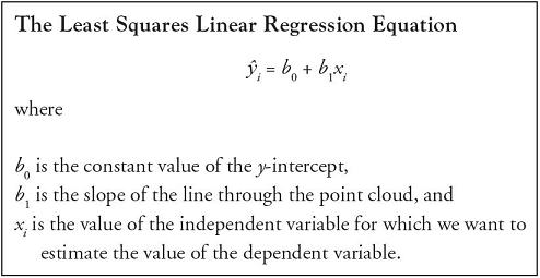
There are many lines that can flow through a cloud of points, so we need a criterion for selecting a specific straight line. The criterion used in simple linear regression is to minimize the squared differences between the actual y-value and the predicted y-value for any given value of x. Hence this line is called the least squares regression line. In this equation, the intercept is b₀, which establishes the location of the point cloud along the y-axis when x has a value of zero, and the slope is b₁, which captures the direction of the point cloud. The subscript “i” denotes that there is a specific x-value along the x-axis for which we want to predict a related y-value, .

In fact, the values reflected in the regression equation can be seen as the sample estimates of their respective population parameters. The value of _i is the estimate based on sample data for the actual values of y_i. The values for b₀ and b₁ are based on the random sample estimating the true population parameters β₀ and β₁, respectively.

Example 8.2.

Use Excel to develop the least squares regression line that uses the annual average 6-month Treasury Bill rates shown in Table 8.1 to predict the inflation rate based on the CPI for urban Americans. If we knew the annual average 6-month Treasury Bill rate was 10%, using the regression line, what would we guess the inflation rate to be?

Answer

Using Excel’s Data Analysis toolkit, the regression analysis for the data produced the output shown in Table 8.1.

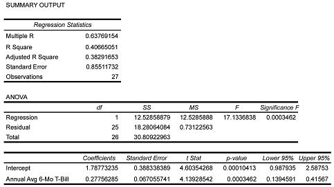
The regression coefficient for the y-intercept, b₀, is 1.7877 and the regression coefficient for the slope, b₁, is 0.2776. The least squares regression line is given as _i = 1.7877 + 0.2776x_i. For x = 10, we would predict the inflation rate to be _i = 1.7877 + 0.2776 • 10 = 4.5634. So, when the annual average Treasury Bill rate is 10%, we would predict the inflation rate to be 4.56%. Note, some differences due to rounding may occur.

Interpretation: The slope of the regression line captures the direction of the point cloud, showing y generally increases 0.2776% for each percent increase in the annual average 6-month Treasury Bill rate. The y-intercept of 1.7877 anchors the regression line at the point (0, 1.7877) and provides the reference point, the beginning of the change captured in the slope, for the location of the point cloud on the y-axis.

To add the regression line to the scatterplot, we simply right-click the mouse on any data point in the plot, click “Add Trendline,” select “Linear,” and indicate that the equation should be shown on the graph. Notice that the linear trendline is the regression line.

The Assumptions of Regression

We have learned to estimate the slope and the y-intercept of the line that best fits the point cloud exhibited by a set of two-dimensional data. If the data points were perfectly predicted by the regression line, all of the points would fall right on that line. But fluctuation is the rule not the exception in sets of real data. The width of the point cloud around the regression line is also an important characteristic to assess in our analysis of the regression model. In general, the more dispersed the point cloud is around the regression line, the less powerful the regression model is in predicting the actual y-values. Conversely, the more narrowly the point cloud aligns around the regression line, the more powerful the regression model is in predicting the y-values.

Four major assumptions underlie the model of simple linear regression:

1. The nature of the relationship between x and y is linear.
2. The errors in y—that is, the differences between the actual value for y and the value for y predicted by the regression line (y_i − _i)—are normally distributed around the regression line for any given value of x_i.
3. The distribution of the errors, those differences between the actual value for y and the value for y predicted by the regression line, (y_i − _i), around the regression line is constant regardless of the value of x.
4. The values of (y_i − _i) are independent of one another and of any given value of x_i.

The errors in estimating each y based on the value of each x are called residuals.

The normal distribution of the errors, or residuals, at any point along the regression line is the same as the normal distribution of the errors at every other point along the regression line. It is as if a single unchanging normal distribution slides along the regression line to generate the errors. The standard deviation of the estimate, s_e, is an estimate based on sample data of the standard deviation of the normal distribution of errors.

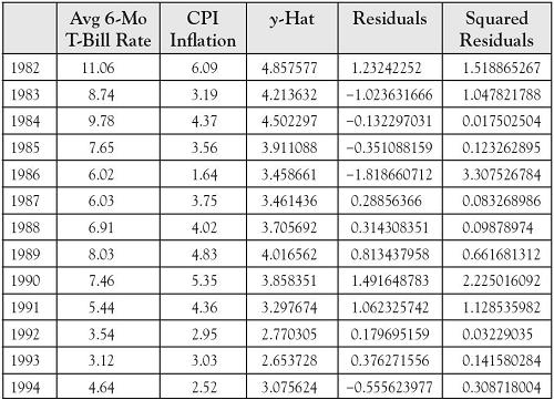
Figure 8.3 contains the calculations for (y_i − _i), the differences between the actual value for y and the value for y predicted by the regression line, where _i = 1.7877 + 0.2776x_i was used to generate the scatterplot in Figure 8.2.

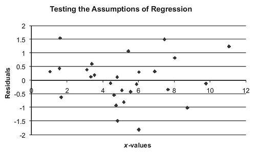
From the values shown in Table 8.3, we form the scatterplot of resulting residuals against the independent variable shown in Figure 8.3. The pattern in Figure 8.3 trends downward for increasing values of the independent variable. Ideally, we would like to see no pattern of increasing or decreasing residuals in the scatterplot. But the regression analysis results are still useful in providing a test of whether there is a relationship between the annual average 6-month Treasury Bill rate and the CPI inflation, and for making improved estimates of CPI inflation based on the value of the annual average 6-month Treasury Bill rate. The scatterplot suggests that the relationship between the annual average 6-month Treasury Bill rate and the CPI inflation may not be a linear relationship. Advanced regression techniques can be used to look at nonlinear models.

The Standard Error of the Estimate

The degree to which the y-values fluctuate around the regression line affects the explanatory power of the analysis. The standard error of the estimate, s_e, is a measure of error generated by using the regression equation, , to predict the actual values of y. Specifically, if the residuals are assumed to be normally distributed, the standard error of the estimate is the standard deviation of those residuals based on the sample data. The further the actual values of y are away from the values of y predicted by the regression equation, the larger is the value of the standard error, s_e. The sum of squared residuals is the core of the error term. The sum of squared residuals divided by the degrees of freedom on error generates the value of SSE, summed squared error, which we find on the Excel printout.

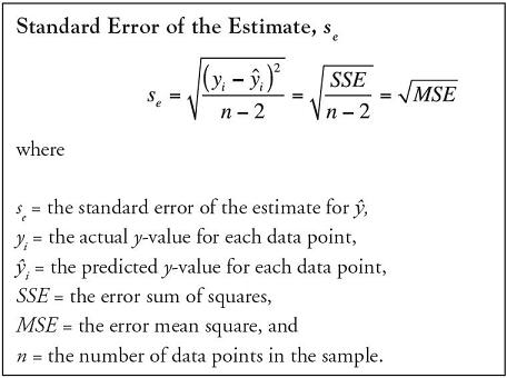
This is the same SSE that we discussed in Chapter 6. The degrees of freedom in simple linear regression are the number of data points minus 2, (n − 2). The ratio of SSE divided by (n − 2) is MSE, and the square root of MSE is called the standard error of the estimate for , or s_e. In terms of our analysis,

The reader can verify the values on the Excel printout contained in Example 8.2.

Using the Regression Model for Estimation

Regression models are useful not only because they provide evidence about the nature and strength of the relationship between two variables. Regression models are also useful because we can use them to make estimates. With the regression model, we can make three kinds of estimates:

1. Individual point estimates of y for a given value of x
2. Interval estimates for the average value of y for all elements of the population that have a given value of the x-variable
3. Interval estimates for an individual value of y for any single element of the population that has a given value of the x-variable

Caution should be used when making any of these estimates with the regression model, however. The model is most accurate for values of x that are close to , the mean x-value. The farther the point of estimation is away from the mean value of x, the less precise is the estimate for the mean of y. Particular caution should be used in pressing a regression model to predict values outside the interval of x-values represented in the observed data.

Point Estimates

Recall that a point estimate is found by substituting the particular value of x into the fitted regression equation to obtain _i, the estimated value of y based on the particular value of x_i. Point estimates are easily computed by calculator or on Excel. The point estimate remains important in all predictions, since it is also the center value of both interval estimates.

Confidence Interval Estimates for the Mean of y

The confidence interval estimate for the mean value of y is used to predict the average or expected value of y for a given value of x = x*.

Example 8.3.

Construct and interpret the 95% confidence interval for the mean inflation rate based on the CPI when the annual average 6-month Treasury Bill rate is 6%.

Answer

We need to accrue all the pieces of information necessary to compute the confidence interval.

_i = 1.7877 + 0.2776x_i = 1.7877 + 0.2776 • 6 = 3.453

t-coefficient for 95% confidence and df = 25 = 2.060

s_e = 0.8551

= 5.25

Lower bound = 3.453 − 0.354 = 3.099

Upper bound = 3.453 + 0.354 = 3.807

Interpretation: Over all years in which the annual average 6-month Treasury Bill rate is 6%, the mean inflation rate based on the CPI will fall between 3.099% and 3.807% with 95% confidence.

Prediction Interval Estimates for Individual Values of y

The prediction interval estimate for the individual value of y is used to predict the particular value of y for a given value of x = x*.

Example 8.4.

Construct and interpret the 95% prediction interval for an inflation rate based on the CPI when the annual average 6-month Treasury Bill rate is 6%.

Answer

Using the same information provided in Example 8.3,

Lower bound = 3.453 − 1.796 = 1.657

Upper bound = 3.453 + 1.796 = 5.249

Interpretation: For an individual year in which the annual average 6-month Treasury Bill rate is 6%, the inflation rate based on the CPI will fall between 1.657% and 5.249% with 95% confidence.

Suppose we had only collected the sample data for CPI inflation (but not for the average 6-month Treasury Bill rate) and wanted to find an interval estimate for the CPI inflation rate next year based on the annual CPI inflation rates between 1982 and 2008. Using the methods from Chapter 3, the point estimate would have been 3.2437% and an interval estimate with a 95% confidence level would have been between 1.006% and 5.481%, using the following calculations:

± t • s = 3.2437 ± 2.056 • 1.089 = 3.2437 ± 2.2390

Comparing this to the prior interval from Example 8.4, we see the regression model creates a narrower, more precise interval estimate for the same level of confidence, along with adjusting the center of the interval estimate based on the association with the 6-month Treasury Bill rate.

Coefficients of Determination and Correlation

While the width of the point cloud around its regression line gives us an insight into how consistent the regression model is in predicting the actual y-values, we do not yet have a method to measure how powerful that relationship is between x and y.

The Coefficient of Determination

An important measure of the strength of the linear relationship between x and y is the percent of the total variation in y that is explained by the variation in x. It is the coefficient of determination, r². Taking advantage of earlier calculations, we define the explained variation in y as the complement of the unexplained variation, or sum of squared residuals.

Example 8.5.

Calculate and interpret the coefficient of determination for the regression of the inflation CPI on the annual average 6-month Treasury Bill rates.

Answer

The coefficient of determination is calculated as follows:

The reader can confirm the value for R Square in the Excel output under “Regression Statistics.”

Interpretation: Nearly 40.7% of the total fluctuation in the inflation rate based on the CPI is explained by changes in the annual average 6-month Treasury Bill rates.

The Coefficient of Correlation

Like the coefficient of determination, the coefficient of correlation, r, is also an important measure of the strength of the linear relationship between x and y. But, in addition to serving as a measure of the strength of the regression model, the coefficient of correlation also reflects the direction of the linear relationship between x and y. It addresses the question: do the annual average 6-month Treasury Bill rates and the rates of inflation based on the CPI increase or decrease in a related way? The coefficient of correlation is related to the coefficient of determination: specifically, the value of the coefficient of correlation is r, the square root of the coefficient of determination, and has the same sign as the slope of the regression model. In terms of the particular data we have been analyzing, the sign of r is positive because the regression slope is positive (b₁ = +0.2776). The value of r is given by the square root of 0.40665, or 0.63769, which the reader can verify is the value for Multiple R in the Excel output under “Regression Statistics.” If the b₁ coefficient in the regression equation had been negative, the coefficient of correlation would have been −0.63769.

Hypothesis Tests for Model Utility

We now have estimates for three of the characteristics important to the linear relationship between the independent variable, x, and the dependent variable, y:

• The y-intercept for the cloud of points, b₀, which estimates β₀
• The direction of the cloud of points, b₁, which estimates β₁, the slope of the regression model, and
• The width of the cloud of points, s_e

We also know how to fit a line through a point cloud using the least squares method. In general, the denser the data points are around the regression line and the steeper the slope of the slope coefficient b₁, the better the regression model is in estimating the value of y. The more dispersed the data points are away from the regression line and the flatter the regression line, the poorer the regression model is in estimating the value of y. We know from the coefficient of determination the percent of total variation in y that is explained by the regression model. What we do not have yet, however, is a tool to tell us how good our regression model is. How close do the data points have to gather around the regression line for us to conclude that our model is doing a better job than simply estimating the value of y based on sample data for the y-variable alone? What amount of confidence can we have in such a conclusion? These are important questions to which we now turn our attention.

The Global F-Test of Model Utility

A test of model utility, or the overall usefulness of the regression model, can be conducted with an F-test. This test answers the question: can we do a better job of predicting actual y-values using the regression model y = than we can by using y = , the average value of y? If the value of y does not depend linearly on the value of x, then the regression line provides an estimate for individual values of y that is no better an approximation of y than the average y-value. Stated alternately, if the value of y does not depend linearly on the value of x, then the regression line, y = , is virtually the same as the line y = . If the regression model is useful, the amount of variance explained by the regression model will be significantly greater than the amount of unexplained variance. Recall from Chapter 6 that the F-statistic is formed by the ratio of two variances, variance that is explained by the variable of interest divided by the unexplained variance. In regression, the F-statistic is formed by the ratio of the mean square regression divided by the mean square error.

Example 8.6.

Looking back on the data from Examples 8.1–8.5, use the global F-test to evaluate whether the regression model y = is a better predictor of the rate of inflation based on the CPI than the horizontal line y = . Use α = 0.05.

Answer

H₀: The regression equation y = is not useful in predicting the actual values for the inflation rates based on the CPI.

H₁: The regression equation y = is useful in predicting the actual values for the inflation rates based on the CPI.

Decision Rule: For α = 0.05 with 1 and (27 − 2) = 25 degrees of freedom for the numerator and denominator respectively, we will reject the null hypothesis if the calculated test statistic falls above F = 4.24.

Test Statistic:

Observed Significance Level: To find an exact p-value for a t statistic, we use Excel’s imbedded function =Fdist(17.1337,1,25), which yields the answer p-value = 0.0003.

Conclusion: Since the test statistic of F = 17.1337 falls above the critical bound of F = 4.24, we reject H₀ with at least 95% confidence. Likewise, since the p-value of 0.0003 is less than the desired α of 0.05, we reject H₀. There is enough evidence to conclude that the regression equation does a better job of predicting the actual inflation rates based on the CPI than using the average inflation rate. The average annual 6-month Treasury Bill rates are useful in predicting the CPI inflation rates.

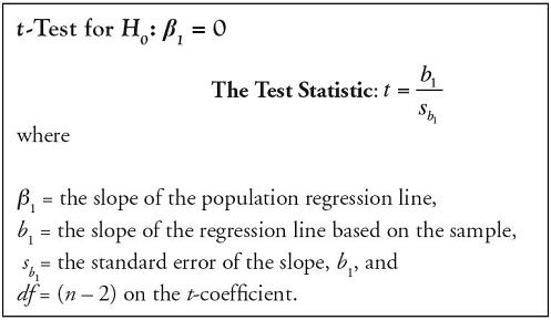
The t-Test for the Slope of the Regression Line

In Example 8.1, we estimated the value of y as if we didn’t know anything about the value of x. To do that, we used the average y-value, or . In fact, this is the basis for the t-test of how well a regression model fits sample data. In simple linear regression, the t-test is a mirror image of the F-test. Since the line y = has a slope m = 0, we can also test the model utility by testing whether the slope of the regression model, β₁, is significantly different from zero. If we are able to reject the null hypothesis, β₁ = 0, then we have evidence that the regression model, y = , is doing a better job of predicting actual values of y than the line y = .

Example 8.7.

Looking back on the data from Examples 8.1–8.5, use the t-test to evaluate whether the regression model y = is a better predictor of the rate of inflation based on the CPI than the horizontal line y = . Use α = 0.05.

Answer

H₀: β₁ = 0

The slope of the population regression line is equal to zero.

H₁: β₁ ≠ 0

The slope of the population regression line is not equal to zero.

Decision Rule: For α = 0.05 with (27 − 2) = 25 degrees of freedom, we will reject the null hypothesis if the calculated test statistic falls above t = 2.060 or below t = −2.060.

Test Statistic:

Observed Significance Level: To find an exact p-value for a t statistic, we use Excel’s imbedded function =tdist(4.139,25,2), which yields the answer p-value = 0.0003.

Conclusion: Since the test statistic of t = 4.139 falls above the critical bound of 2.060, we reject H₀ with at least 95% confidence. Likewise, since the p-value of 0.0003 is less than the desired α of 0.05, we reject H₀. There is enough evidence to conclude that the regression equation does a better job of predicting the actual inflation rates based on the CPI than using the average inflation rate. The average annual 6-month Treasury Bill rates are useful in predicting the CPI inflation rates.

Comparing the Global F-Test and the t-Test of Model Utility

It is a reasonable question to ask: what is the relationship between the global F-test and the t-test of the regression coefficient just completed? In simple linear regression, the two tests mirror one another. Notice that the p-value on the t-test is the same as the p-value on the F-test. Both p-values are reported as 0.003462. In fact, the square of the t test statistic, 4.139, equals the F test statistic, 17.1337. The square of the t critical bound, 2.060 or more precisely 2.0595, is the F critical bound, 4.24 or more precisely 4.2417. Both values were rounded and reported here as 2.060 and 4.24. In multiple regression, where more than one independent variable is included in the analysis, the t-test of individual regression coefficients and the global F-test part ways and serve separate purposes. Multiple regression models are not covered in this text.