Chapter 3

Understanding the Normal Distribution and the t-Distribution

If you have ever watched someone sift flour in a kitchen or dig a hole and pile the dirt in the same place outside, you have seen a normal distribution, albeit somewhat imperfect. It is bell shaped, symmetric, peaked in the center with tails that trail off rapidly the greater the distance from the center. While imperfect versions of the normal distribution are easily seen in ordinary life, its discovery is credited to the great German mathematician Johann Carl Friedrich Gauss (1777–1855), who documented that errors of routine measurements often follow a normal distribution. Some normal distributions can be huge, as seen in a pile of hulls at the end of a dump chute from an almond hulling plant, for example, and others quite tiny in comparison. Normal distributions occur because the greatest numbers of elements in the “pile” fall straight down below the location of the end of the chute or the bottom of the sifter or the tip of the shovel. Some elements tumble off center, down the growing sides of the “pile.” Unless otherwise constrained, occasionally an element will tumble relatively far away from the center. Because the height, μ, and breadth, σ, in different distributions can differ over many magnitudes, the standard normal distribution is introduced to standardize their discussion.

The Standard Normal Distribution

All normal distributions share the same shape, differing only by the location of the center and the degree of spread. The standard normal distribution is the normal distribution that has a mean of 0 and a standard deviation of 1. The axis along the bottom of the distribution represents the number of units of standard deviation a particular value is above or below its mean, which is called the z-score.

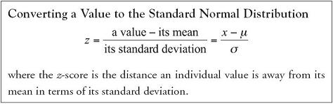
The standard normal distribution is useful because its table details the amount of area captured under the normal curve below a given value. The reason we care about the amount area captured under a normal curve is that it represents the likelihood that a value will fall within a defined segment of a normal distribution. Any normal distribution can be converted to the standard normal distribution by subtracting the value of its mean (or center point) and then dividing that difference by the standard deviation for the population. The Standard Normal Table converts the linear distance a value is away from its mean on the bottom axis of the distribution to the likelihood that a value will fall that far or less away from its mean, which is the area captured under the normal curve below that value. Let’s investigate a few elementary examples.

Example 3.1.

What is the probability that a z-score will fall below a score of 1.04?

Answer

Locate the ones and tenths digits as a row header on the cumulative standard normal distribution. Locate the hundredths digit as a column header on the table and trace down the column and across the row identified to find their intersection. See Table 3.1. The answer is

P(z < 1.04) = 0.8508

Interpretation: Approximately 85.08% of the area under a normal curve will fall to the left of a z-score of 1.04. There is an approximate 85.08% chance that an element randomly selected from a normal population will fall below a z-score of 1.04.

Example 3.2.

What is the probability that a z-score will fall above a score of 1.04?

Answer

Using the same area found in Table 3.1, since we want the area above the given z-score, we subtract that area from 1. The answer is

1 − P(z < 1.04) = 1 − 0.8508 = 0.1492

Interpretation: Approximately 14.92% of the area under a normal curve will fall to the right of a z-score of 1.04. There is an approximate 14.92% chance that an element randomly selected from a normal population will fall above a z-score of 1.04.

A special note is worth making at this point of our discussion. Sometimes we talk about z-scores that are strictly less than a given value, as we did in Example 3.1. Other times we talk about z-scores that are less than or equal to a given value. While the difference can be captured in notation mathematically,

P(z < 1.04) versus P(z ≤ 1.04)

computationally there is no difference in the probability satisfying the two depictions. The reason is that a point has no breadth or depth. So an individual point, in this case z = 1.04, has no dimension and carries with it no area under the curve. You might recall that a geometric boundary that is excluded from an area is shown with a dotted line, and a boundary that is included in an area is shown with a solid line. But the inclusion of the single boundary point, and therefore its edge, makes no difference to the calculation of the area itself.

Standardizing Individual Data Values on a Normal Curve

Not all variables are normally distributed. Many events we can think of are skewed, like personal income or residential housing prices. However, if a variable is normally distributed, we can analyze its distribution through the standard normal distribution using the following equation:

Let’s consider an example.

Example 3.3.

Suppose we know that delivery times for an interstate package shipment company are known to be normally distributed with a mean of 3.5 days and a standard deviation of 0.8 days. What is the probability that a package will take more than 5 days to be delivered?

Answer

The individual package delivery time in question is 5 days, with a mean delivery time of μ = 3.5 days and a standard deviation of σ = 0.8 days.

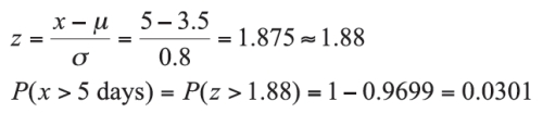
Interpretation: There is a slightly better than 3% chance that a package will require more than 5 days to be delivered by this company. While it is possible that a package will require more than 5 days to deliver, it is highly unlikely.

The t-Distribution

The Student’s t-distribution, also known simply as the t-distribution, is bell-shaped, like the standard normal distribution. Like the standard normal distribution, the t-distribution also represents the distance a value is above or below its mean in terms of its standard deviation and converts that distance into the area under the curve beyond that value. In contrast, however, the t-distribution is less concentrated around the mean and has thicker tails than the z-distribution. In fact, the t-distribution is a family of curves that is flatter the smaller the sample size and that becomes more centrally mounded the larger the sample size. Fundamental to this dynamic is the notion of degrees of freedom (df), which is a measure of the strength of the sample in estimating the population mean. When estimating the value of a mean, we have (n − 1) additional elements to support and refine the value of the first sampled element. Seen another way, once we know the mean of the sample, we only need to know (n − 1) elements in the sample and the value of the remaining element is determined. So we have (n − 1) degrees of freedom in the sample to estimate the mean.

Because the shape of the curve actually changes for each change in the degrees of freedom, a separate table for each df would be required to have the distribution fully displayed. To economize, the values for frequently used areas are extracted and displayed in a table for the t-distribution. Using the table for the t-distribution, then, requires we identify the degrees of freedom and the particular area of interest to find the t-coefficient, which is the number of units of standard deviation a value would be away from its mean in order to capture the desired area. To find the t-coefficient, for example, that marks off 10% of the area in the upper tail of the t-distribution for df = 35, we locate the column headed by α = 0.10 and run across the row headed by df = 35 to find the value t = 1.306. An example, Example 3.4., will be developed later in the chapter using the t-distribution.

Understanding the Behavior of Sample Means

One of the main reasons we study samples from populations is because we want to estimate a population parameter like the mean. If we randomly gather one sample and compute its sample mean, and then randomly gather another sample and compute its sample mean, we will generally get different sample mean values. Further, it is highly unlikely any particular sample mean will be the true population mean, μ.

We take samples and infer back to what the samples say about the population they could have come from. In fact, if we took many samples and determined their sample means, the mean of all sample means taken from the population is the population mean itself: . The set of sample means for all possible samples of size n taken from a population defines a probability distribution referred to as the distribution of sample means or the sampling distribution of .

Error is inherent in the process of taking repeated samples. Inferences are, after all, based on incomplete data. The difference between the sample statistic and the population parameter it estimates is called the sampling error. We need to allow for error in our estimate of the population parameter. It can be shown mathematically that the standard deviation of the sampling distribution of the mean, the standard error, is given by 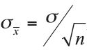, where σ is the population standard deviation and n is the sample size.

Regardless of the sample size, the center of the sampling distribution of the mean is always the population mean: . Put another way, the center of the sampling distribution of the mean is not sensitive to the sample size. However, the standard deviation of the sampling distribution of the mean is sensitive to the sample size. The larger the sample size, n, the more similar the sample means will be and the more concentrated the sample means will be around the true population mean. In other words, the larger the sample size, the smaller the standard error and the more “peaked” or “mounded” the sampling distribution will be around the population mean; the smaller the sample size, the larger the standard error and the “flatter” or less concentrated the sampling distribution will be around the population mean.

When the Population Distribution Is Normal and σ Is Known

The sample size does not affect the location of the center of the sampling distribution, but it does affect the shape, the “moundedness,” of the sampling distribution. The larger the sample size, the more concentrated, the more “mounded,” the sampling distribution of the mean becomes. How mounded the sampling distribution becomes is important for us to know in determining if the normal distribution is a good fit for our sampling distribution. Knowing that the sampling distribution is normally or approximately normally distributed is important because we can standardize the sample mean with reference to the standard normal distribution using the following equation.

When the Shape of the Distribution Is Unknown or Known to Be Not Normal

If the shape of the underlying population is either unknown or is known to be not normal, the sampling distribution of sample means may still be approximately normally distributed, but only when the sample size, n, is sufficiently large. If the sample size is sufficiently large, the sampling distribution of the mean is sufficiently concentrated around the mean that the sampling distribution is approximately normally distributed. Known as the Central Limit Theorem, the principle dynamic depends on the sample size, n.

There are a number of qualifiers in our language here: “sufficiently,” “approximately,” “nearly.” They play an important role in capturing the dynamic relationship between sample size, n, and the resulting shape of the sampling distribution of all sample means based on n elements. It is an important dynamic to understand because the sample size is most often a decision variable for the researcher to set. The sample size can be set at the beginning of data collection so that the resulting sample mean can be compared to a nearly normal distribution for analysis. How large does a sample size have to be so the researcher can be relatively confident the resulting sample mean can be compared to an approximately normal distribution? It can be shown mathematically that, for most populations, if the sample size is at least 30, the resulting sample mean can be compared to an approximately normal distribution.

In most applications of statistics, the population variance is not known. When the population variance is not known, two elements take on increased importance: the shape of the underlying population that was sampled and the size of the sample taken. As long as the underlying population is not heavily skewed and as long as the sample size is sufficiently large to satisfy requirements of the Central Limit Theorem, the t-distribution will be a good approximation of the sampling distribution, which uses the sample standard deviation, s, in place of the population standard deviation, σ.

The larger the sample size n is, the better the approximation the t-distribution with (n − 1) degrees of freedom is for the distribution of sample means. If the underlying population is not normal but is not heavily skewed, the t-distribution remains a reasonably good approximation of the sampling distribution of the mean as long as the sample size is sufficiently large to invoke the Central Limit Theorem.

Let’s consider an example.

Example 3.4.

Suppose the average hourly production for a sample of 50 hours of assembly operations was 159.32 units with a standard deviation of 17.6. If the mean production level were actually 165 units per hour, how likely is it that we would get a sample of 50 hours with an average of 159.32 units or less?

Answer

The population hourly production level, or μ, is 165 units per hour. A sample of n =50 hours of assembly operations represents = 159.32 with a sample standard deviation of s = 17.6 units per hour.

The t-coefficient falls between t_.01 = −2.407 and t_.025 = −2.010. From the t-table, all we can say is that the probability falls between 0.01 and 0.025. Using Excel, we can use the TDIST function to determine the exact value of the probability at 0.013434.

Interpretation: There is a 1.34% chance that a sample of 50 hours will produce an average hourly production of 159.32 units or less when the true population mean production is 165 units per hour. While it is possible that the average hourly production level of 159.32 units or less can occur when the real population production level is 165 units per hour, it is not very likely to occur.

Understanding the Behavior of Sample Proportions

Measurements generate continuous quantitative data that are typically summarized with means and standard deviations. Counts are discrete data typically summarized with proportions. Theoretically, the appropriate distribution for discrete data is a member of the set of discrete distributions. Discrete distributions are complex to work with computationally, however, and it has been shown that if the sample sizes are sufficiently large, the z-distribution is a very good approximation of the sampling distribution of the proportion that is created by a ratio of the counts generated.

To reasonably estimate a discrete distribution with the z-distribution, the sample size must be large enough for the product of n • p and n • (1 − p) to be greater than or equal to 5. Realistically, only the smaller of the values p and (1 − p) must be tested. The closer the population proportion is to 0.5, the smaller the required sample size is to meet the conditions stated above. For example, if p = 0.5, a sample size of 10 would be sufficient. If p = 0.1, however, a sample size of at least 50 is required. If p = 0.8, a sample size of at least 25 would be required, since (1 − 0.8) = 0.2 and 0.2 × 25 = 5.

Let’s consider an example.

Example 3.5.

According to the Food Marketing Institute, approximately 22% of all grocery shoppers do most of their shopping on Saturday. How likely is it that a random sample of 72 shoppers indicates that fewer than 12% do their grocery shopping on Saturday?

Answer

The sample proportion is 12%, the population proportion is 22%, and the sample size is 72.

Interpretation: There is a 2% chance that a sample of 72 homes will produce a sample proportion of 12% or less who do most of their grocery shopping on Saturday. While it is possible that the proportion of shoppers will have 12% or less who do most of their grocery shopping on Saturdays, it is not very likely to occur.

Point and Interval Estimates

Sometimes what we need is a good estimate of the value for an important variable. How much income do we anticipate generating during the next fiscal year? What proportion of a region’s population served by the community’s hospital will require emergency room treatment during the next month? A point estimate is the single value that best approximates the value of a population parameter of interest. If we take a random sample from a population and compute the sample mean, , this would serve as a point estimate of the true population mean, μ. If we want to estimate the proportion of a population that falls in a particular category, the sample proportion, , would serve as the point estimate of the true population proportion, p.

In contrast, an interval estimate is a set of numbers centered at the point estimate and extending above and below the point estimate. Because of sampling error, we know a sample statistic will not be exactly equal to the parameter it estimates. An interval estimate allows for the occurrence of sampling error. More exactly, an interval estimate is constructed from n sample data in a way that a specified percent of all possible samples of size n taken from the same population will contain the true value of the population parameter.

Under certain assumptions, using a z- or t-coefficient allows us to accommodate and control for the sampling error in our estimates of the population mean or proportion. Earlier in this chapter, we calculated the z- or the t-value based on data from the sample to determine the probability that the sample statistic would fall in a certain range. Here, our use of a particular z- or t-coefficient is to determine a likely range for our estimate of the population mean or proportion. The coefficient is derived from the appropriate table based on the amount of confidence we want to have that our interval will contain the true population mean or proportion. The amount of risk we are willing to sustain is 100(α)%, and the amount of confidence we want to have is 100(1 − α)%, where α is pronounced alpha. We will expand our discussion and use of alpha in Chapter 4.

Confidence Intervals on the Mean

Algebraically we can derive the equation for the confidence interval for a mean from the equation we used earlier to standardize means. We begin with the definition of the z-coefficient, . We then multiply both sides of the equation by the denominator of the right-hand side, , which is the standard error of the mean,

arriving at the equation for the z-confidence interval, . The equation for a t-confidence interval can be derived in the same way, giving us the equation for the t-confidence interval, .

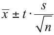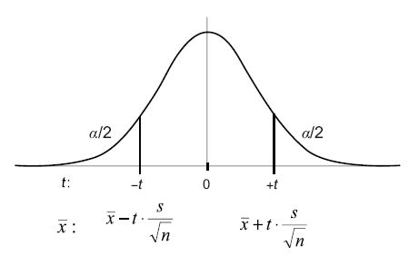
Geometrically, the structure of the interval is perhaps more easily understood. The product of the z- or t-coefficient times the standard error of the mean is actually the distance between the center of the interval, in this case , and either the upper or the lower interval bound. Two times that product is the width of the entire interval, so the product of the z- or t-coefficient times the standard error of the mean is called the interval half-width. The lower bound of the confidence interval is the point estimate minus the interval half-width and the upper bound of the confidence interval is the point estimate plus the interval half-width.

We can construct an interval that functions in essence as a measuring tape, so that, between its lower and upper bounds, the population parameter will fall in a stated percent of all possible sample intervals of size n taken from that population. If we want to be 100(1 − α)% confident that samples of a certain width will contain the population parameter, then we select the z- or t-coefficient associated with that level of confidence. Alternatively, we can conclude that, over a large number of repeated samples of the same sample size n, 100(1 − α)% of the sample means will fall between the lower and the upper confidence interval bounds.

For z-confidence intervals, the population standard deviation, σ, must be known and either the underlying population being sampled is approximately normally distributed, or the sample size n must be sufficiently large to invoke the Central Limit Theorem. For t-confidence intervals, the population standard deviation, σ, is not known, so we use the sample standard deviation, s, in its place. Additionally, the underlying population being sampled must be normally distributed. In both confidence intervals, the samples must be randomly chosen for any inference to hold about the population being sampled.

Example 3.6.

A food processing company makes tortilla chips. Although its 16-ounce bags of chips are routinely sampled for compliance with the stated product weight, the company has recently renewed sampling individual bags for the number of chips each contained. Historic data indicate the number of chips per bag is normally distributed with a standard deviation of 38. A random sample of 50 16-ounce bags taken from yesterday’s production run yielded a sample mean of 176.4 chips per bag. Between what two bounds on the number of tortilla chips per 16-ounce bag can we be 95% confident that the interval contains the true process mean?

Answer

Because the population standard deviation is given (σ = 38) and the population is known to be normally distributed, we will use a z-confidence interval to establish bounds on the mean number of chips per 16-ounce bag. To be 95% confident, the 5% risk we are wrong is split between the upper and lower tails of the distribution. The appropriate z-coefficient is z = ±1.96. The sample size is given, n = 50, and the sample mean is given, = 176.4.

Upper bound:

Lower bound:

Interpretation: We can be 95% confident that if we tested all bags of tortilla chips, the true mean number of chips per bag will fall between 165.87 and 186.93.

Confidence Intervals on the Proportion

Algebraically we can derive the equation for the confidence interval for a proportion much as we did for the confidence interval on a mean, with one significant difference. We are working with sample data only, so the standard error of the proportion, , is formed on the sample proportion: , which leads us to the equation for the z-confidence interval, .

Example 3.7.

A manufacturer of drip irrigation controllers is interested in reporting an interval estimate for the proportion of manufactured units that are defective. A random sample of 800 controllers determined that 12 were defective. Between what two bounds can we be 90% confident that the interval estimate contains the true defective rate for all drip irrigation controllers?

Answer

Since the number of defective controllers (12) and the number of fully functional controllers (788) are both greater than 5, we will use a z-confidence interval to establish bounds on the defective rate. To be 90% confident, the 10% risk we are wrong is split between the upper and lower tails of the distribution. The appropriate z-coefficient is z = ±1.645. The sample proportion is found by dividing the number of defective controllers by the overall sample size, .

Upper bound:

Lower bound: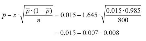

Interpretation: We can be 90% confident that if we tested all irrigation controllers, the defective rate will fall between 0.8% and 2.2%.