Chapter 5

Testing Two Population Means and Proportions

The ability to compare two population parameters is both useful and important in expanding the roles estimation and hypothesis testing can play in analyzing sample data. In this chapter, we continue our discussion of population means, variances, and proportions, but we develop the analysis to compare differences between two population means and differences between two proportions. The underlying logic of hypothesis testing remains unchanged.

We encounter several complexities in expanding our analysis to two populations that we did not find in dealing with a single population. In analyzing differences between population means, we separate those that are estimated with independent samples taken from two unrelated populations and those that are estimated with dependent samples taken from two closely related populations. Samples taken from two populations are independent when a random sample of elements is drawn from each population separately. If, on the other hand, we construct samples so that each element in the sample from one population corresponds to, or is paired with, an element in the sample from the second population, we have dependent samples. We continue to work with the z- and the t- distributions but find there are two different t-tests to use depending on whether the population variances are equal or unequal.

The t-Test for Differences Between Two Means Given Independent Samples and Equal Variances

We introduce the t-test first because it is so frequently used. More often than not, we deal with samples taken from populations for which we do not know their population standard deviation, σ. The t-test is considered a robust test even if the underlying populations are not normal because it still generates reasonably accurate results if the sample sizes are large enough to invoke the Central Limit Theorem.

Inferences about the difference between population means (μ₁ − μ₂) taken from two independent samples are based on two random samples from two unrelated populations. The two samples do not have to be the same size, and nothing about the way in which one sample is selected from the first population affects the elements that are sampled from the second population. Because we are estimating two population parameters, the degrees of freedom for use with the t-distribution are combined from each of the samples: df = (n₁ − 1) + (n₂ − 1), or df = (n₁ + n₂ − 2).

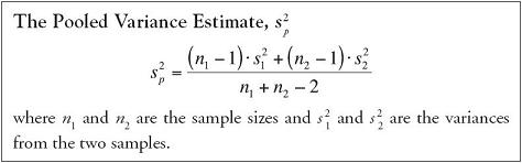
Later in this chapter, we will discuss a statistical test to settle the question of whether two population variances are different enough that we should consider them unequal. For this text section, we will assume the population variances are roughly equal. So, given we assume the two variances are equal, we act accordingly. We combine the two sample variances and form a single pooled variance estimate, s² _p, which is the two sample variances weighted, or multiplied, by their individual degrees of freedom and averaged across their combined degrees of freedom.

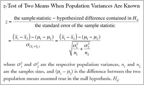
The test statistic is determined by the same general equation we have seen in previous chapters

Usually we are testing the question of whether there is any difference between the two means, so (μ₁ − μ₂) is usually zero, which simplifies the computation a bit.

Example 5.1.

A diversified company set up separate e-commerce sites to handle orders for two of the company’s product lines. Internal auditors randomly selected 32 one-hour periods when they recorded the number of orders placed on site A and 36 periods when they recorded the number of orders place on site B. Summary statistics for the number of orders recorded are as follows:

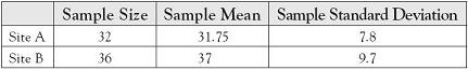
Assuming equal variances, is there sufficient evidence at the 5% level of significance to conclude that the two sites differ in the average number of orders they generate hourly?

Answer

H₀: μ_A − μ_B = 0
There is no difference in the average number of orders generated on the two sites.

H₁: μ_A − μ_B ≠ 0
There is a difference in the average number of orders generated on the two sites.

Decision Rule: For α = 0.05 and df = 32 + 36 − 2 = 66, we will reject the null hypothesis if the calculated test statistic falls above t = 1.997 or below t = −1.997. See Table 5.1.

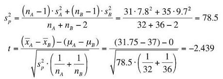
Test Statistic: First, compute the pooled variance estimate, then use that estimate to calculate value of the test statistic.

Observed Significance Level: To find the p-value for the t test statistic, we use the function in Excel =tdist(2.439,66,2). Note that the tdist function of Excel allows us to include the fact that there are 2 tails (the last number in the parentheses), so we do not have to double the area to find a full p-value. As an aside, the tdist function does not accept negative values for the test statistic, so we need to take the absolute value of t = −2.439 as an input to the Excel function.

p-value = 0.0175

Conclusion: Since the test statistic of t = −2.439 falls well below the lower critical bound of t = −1.997, we reject H₀ with at least 95% confidence. Likewise, since the p-value of 0.0175 is less than the desired α of 0.05, we reject H₀. There is enough evidence to conclude that the two web sites differ in the average number of orders they generate hourly.

A final note on Example 5.1. is appropriate before we proceed. We may be tempted to conclude that Site A had a smaller average number of orders per hour than Site B. After all, we might rationalize, that is what the sample data say. But we can only speak to the hypothesis that we formed at the beginning of the experiment, which in this case was around the question of whether there was any difference between the two means. If we overstep our original hypothesis, we will underestimate the risk we have in drawing the final conclusion.

The t-Test for Differences Between Two Means Given Independent Samples and Unequal Variances

When the two populations of interest are nearly normal but we conclude their variances are not equal, differences in their sample means can be approximated by a t-distribution, although the degrees of freedom differ from those we used in the equal-variances t-test. The calculations for the degrees of freedom to be used in the unequal-variances t-test are complex, as shown in the equation that follows, but are easily found in the automated analysis provided routinely by Excel.

Example 5.2.

A package handler has two offices in the same city. A recent sample of 30 randomly selected customers at the western office indicated that their average wait time for customer service is 5.6 minutes with a standard deviation of 2.24 minutes. During the same time period, a sample of 35 randomly selected customers at the central office indicated that their average wait time for customer service is 7.4 minutes with a standard deviation of 3.78 minutes. Use the unequal variances t-test to determine whether there is any difference in the average wait times for customer service at the two offices. Use α = 0.05.

Answer

H₀: μ_W − μ_C = 0
There is no difference in the average wait time for customer service at the two offices.

H₁: μ_W − μ_C ≠ 0
There is a difference in the average wait time for customer service at the two offices.

Decision Rule: Before we can determine the critical bound in t, we need to compute the degrees of freedom to use in finding the critical bound. Note that the calculation for df uses sample variances, not sample standard deviations.

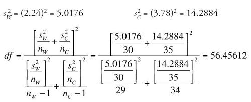
So, using only the integer portion of the final answer, we will use df = 56. For α = 0.05 and df = 56, we will reject the null hypothesis if the calculated test statistic falls above t = 2.003 or below t = −2.003.

Test Statistic:

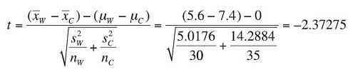
(We show the full decimal values for the calculations for df and the test statistic in case you want to track the calculations yourself.)

Observed Significance Level: To find the p-value for the t test statistic, we use the function in Excel =tdist(2.37275,56,2).

p-value = 0.0211

Conclusion: Since the test statistic of t = −2.373 falls well below the lower critical bound of t = −2.003, we reject H₀ with at least 95% confidence. Likewise, since the p-value of 0.0211 is less than the desired α of 0.05, we reject H₀. There is enough evidence to conclude that there is a difference in the average wait times for customer service at the two offices.

The F-Test for Equality of Two Variances

When we sample randomly from the same population, sample variances do vary simply because we randomly select different subsets of the population. But how different do variances have to be before we are concerned that they are not equal? To test the equality of population variances, whether σ²₁ = σ²₂, we form the ratio of the two variances by dividing both sides of the equation by one of the variances. We then determine if the resulting ratio is significantly different from 1. The best estimate for is the ratio of the two related sample statistics . When two independent samples are taken from normally distributed populations with equal variances, the sampling distribution of their ratios follows an F-distribution, named after the English statistician Sir Ronald A. Fisher (1890–1962). The F-distribution includes the degrees of freedom for each of the two samples: n₁ − 1 degrees of freedom for the numerator and n₂ − 1 for the denominator.

Finding the upper critical bound for the hypothesis test of the F-ratio is relatively straightforward: find the F-ratio, , for with n₁ − 1 degrees of freedom for the numerator and n₂ − 1 degrees of freedom for the denominator. Finding the lower critical bound for the F-ratio is more complex. Because the F tables were generated under the assumption that σ²₁ > σ²₂, to find the lower critical bound of the F-ratio, we must switch the degrees of freedom and find the inverse of the F-ratio, , for that has n₂ − 1 degrees of freedom for the numerator and n₁ − 1 degrees of freedom for the denominator. We often find it more convenient to form the null and alternative hypotheses with the larger of the two sample variances in the numerator. In doing so, we force the comparison of the F test statistic with the upper critical bound of the decision rule, which is the easier of the two bounds to form.

To find the appropriate critical bound from the F-table, we first determine the amount of area in the upper tail of the desired rejection region. If we are conducting an equality test of variances using α = 0.01, the appropriate table to use shows 0.005 in the upper tail. If we were conducting an equality test of variances using α = 0.05, then the appropriate table to use shows 0.025 in the upper tail. The numerator degrees of freedom head the columns across the top of the table and the denominator degrees of freedom head the rows down the side of the table. As an example, for numerator df = 24, denominator df = 30 in an equality test of variances using α = 0.05, we would access the F-table for 0.025 area in the upper tail and find the F = 2.14. See Table 5.2.

Example 5.3.

A random sample of recent graduates from an MBA program was asked about their first-year salary after graduation. Responses were separated by gender and summarized:

Use α = 0.05 to determine whether the variance among the women’s salaries was significantly different from the variance among the men’s salaries.

Answer

The variances among women’s and men’s salaries are approximately equal.

The variances among women’s and men’s salaries are not equal.

Decision Rule: To determine the upper critical bound, we use the numerator df = 30, denominator df = 40, and = 0.025 to find F = 1.94. To determine the lower critical bound, we use the numerator df = 40, denominator df = 30, and = 0.025 to find F = = 0.498. So we will reject the null hypothesis if the calculated test statistic falls above F = 1.943 or below F = 0.498.

Test Statistic:

Observed Significance Level: To find the p-value for the F test statistic, we use the function in Excel =2*Fdist(3.231,30,40). We have to double the output from the Fdist function because it assumes a one-tailed test.

p-value = 0.0006

Conclusion: Since the test statistic of F = 3.231 falls well above the upper critical bound of F = 1.943, we reject H₀ with at least 95% confidence. Likewise, since the p-value of 0.0006 is less than the desired α of 0.05, we reject H₀. There is enough evidence to conclude that the variances among women’s and men’s first-year salaries are not equal. With this result, we would be warranted to use the t-test assuming unequal variances when we test for any difference in the two population means.

The z-Test for Differences Between Two Means Given Independent Samples

In some circumstances, the variances of population parameters are known. Practically speaking, this is true of highly automated processes where the parameters being measured are components of process specifications or where the measurements are taken from a stable historic process. When the population variances are known and the populations themselves are normally distributed, differences in their sample means can be approximated by the standard normal distribution, the z-distribution, regardless of the sizes of the samples taken. When the population variances are known and the sample sizes are sufficiently large, differences in their sample means can be approximated by the standard normal distribution, the z-distribution, regardless of the shapes of the underlying populations.

Example 5.4.

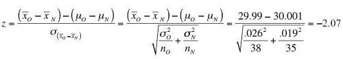
A food processor recently expanded production at their base plant in Oakville by adding a new and more technologically advanced fill line. The older line is known to maintain a mean fill of 30 ounces with a standard deviation of 0.026 ounce. The newer line has a mean fill of 30 ounces with a standard deviation of 0.019 ounce. Use the following sample data to determine whether the new line differs in average fill from the older line. Use α = 0.05.

Answer

H₀: μ_O − μ_N = 0
There is no difference in the average product weight for the two fill lines.

H₁: μ_O − μ_N ≠ 0
There is a difference in the average product weight for the two fill lines.

Decision Rule: For α = 0.05, we will reject the null hypothesis if the calculated test statistic falls above z = 1.96 or below z = −1.96.

Test Statistic:

Observed Significance Level:

p-value = 2(0.0197) = 0.0384

Conclusion: Since the test statistic of z = −2.07 falls below the critical bounds of z = −1.96, we reject H₀ with at least 95% confidence. Likewise, since the p-value of 0.0384 is less than the desired α of 0.05, we reject H₀. There is enough evidence to conclude that the two fill lines have a different average product weight.

The t-Test for Differences Between Two Means Given Dependent Samples

Selecting pairs of similar elements and then submitting each of the pair to different experimental treatments is one of the most powerful research designs available. When facing a difficult decision, who wouldn’t love to identify a pair of clones and send each on different paths into the future to know which path had the better outcome? The analysis of matched pairs is a powerful design for the very reason that the researcher is able to hold all other characteristics constant and focus solely on the effect of the different treatments.

As we have seen in prior sections of this chapter, the comparison of independent samples assumes that the samples are randomly selected and represent the heterogeneity inherent in each of the two populations. Because they are randomly selected, the samples, in essence, are little microcosms of each of the underlying populations. In contrast, dependent samples represent a random sample from one population but a controlled sample from a second population. Once the sample is selected from the first population, elements included in the second sample are in some way either dictated or constrained by the identity of the elements in the first sample. The design of the research plan for two means given dependent samples is itself made more complex by the process required to identify matched pairs of elements, or “clones.” The process of matching elements from one population with elements selected from another population is difficult when such twins do not occur naturally. Pairing observations taken from the same individual before and after a treatment is among the simpler designs using dependent samples. Matching pairs can be both extensive and invasive if the design requires, for example, genetic or psychological profiles of central characteristics. Of essence in the identification of matched pairs is the fact that elements in a second sample are selected precisely because they mirror elements in the first sample. The samples are in no way independent of one another.

Not only is the research design for matched pairs different from that used in identifying independent samples, but the analysis of the results also differs from what we have seen in prior sections of this chapter. In matching the pairs of observations, we analyze the differences observed across each pair by forming the mean and standard deviation of the differences noted for each paired set of observations. As long as the populations being sampled are approximately normally distributed, analysis of the average difference then closely tracks the t-test conducted on one-population parameters as performed in Chapter 4.

There is an important toll paid for designing a paired difference analysis as opposed to an analysis of two independently selected samples: the degrees of freedom on the associated t-statistic are half the size of the degrees of freedom for independently selected samples. Note that the degrees of freedom for a t-test for the mean difference of two dependent samples is the number of pairs of observations minus one rather than the independent sample sizes added together minus two. In exchange for the loss of degrees of freedom, however, the successful paired differences t-test reduces sources of fluctuation that occur from extraneous influences within the variable being measured and focuses the standard error on the differences between the paired observations.

Example 5.5.

Before releasing an advertisement for a new product, the advertising executive for a major fast food chain planned to collect sales data from 25 franchises in the region to track the effectiveness of the new campaign. He selected two dates, one before release and one after release of the advertisement, and requested daily sales totals from each of the 25 outlets. Summary statistics are as follows:

_D = $52.48 s_D = $132.5378

Assuming the populations sampled are approximately normally distributed, is there sufficient evidence to show that the new campaign was effective in increasing the daily sales revenues for franchises in the restaurant chain? Use α = 0.05.

Answer

H₀: μ_After − μ_Before* ≤ 0
The new advertising campaign was not effective in increasing the daily sales revenues for franchises in the chain.

H₁: μ_After − μ_Before* > 0
The new advertising campaign was effective in increasing the daily sales revenues for franchises in the chain.

*Instead of using a single expression, μ_D, to refer to the difference, we show the expression (μ_After − μ_Before) to indicate the order in which the difference was calculated. To be clear, (μ_After − μ_Before) = μ_D.

Decision Rule: For α = 0.05 and df = 25 − 1 = 24, we will reject the null hypothesis if the calculated test statistic falls above t = 1.711.

Test Statistic:

Observed Significance Level: To find the p-value for the t test statistic, we use the function in Excel =tdist(1.9798,24,1).

p-value = 0.02965

Conclusion: Since the test statistic of t = 1.9798 falls above the critical bound of t = 1.1711, we reject H₀ with at least 95% confidence. Likewise, since the p-value of 0.02965 is less than the desired α of 0.05, we reject H₀. There is enough evidence to conclude that the new advertising campaign is effective in increasing the daily sales revenues for franchises in the chain.

The z-Test for Differences Between Two Proportions

As municipal, state, and national election polls predict popular support for favored candidates and causes, the estimation and comparison of population proportions play an important role in anticipating and expressing the voice of the people and their democratic decisions. Preelection polls boast support for this or that candidate or cause at a certain level, within plus or minus a stated percent. There are few statistical topics as widely publicized or as important to the conduct of political processes as the estimation and comparison of population proportions. The difference between two population proportions plays an equally important role in business, in market research, business forecasting, financial auditing, and analysis of comparative defect rates, to name a few. At the heart of the proportion is a count, not a measurement, of sampled elements. When we sort a sample into subgroups—those elements that do meet a certain criterion and those that do not—and then produce a count of these subgroups, we use a proportion to compare the results.

Inferences about (p₁ − p₂) are based on two random samples from two unrelated populations. The two samples do not have to be the same size. We summarize the sample statistics for each, including sample sizes, the number of successes in each sample, and the sample proportions. The best estimate for the population parameter (p₁ − p₂) is the sample statistic (₁ − ₂), where p₁ is the proportion for population 1, p₂ is the proportion for population 2, ₁ = is the proportion for sample 1, and ₂ = is the proportion for sample 2. Since we assume the population proportions are equal in the null hypothesis, we combine the two samples and form a single pooled estimate of the population proportion, _pooled = , which we use in the calculation of the test statistic, if the sample sizes are sufficiently large.

If the sample sizes are sufficiently large, the sampling distribution of (₁ − ₂) can be approximated by the standard normal, or z, distribution. As with the considerations for a single population proportion, what constitutes “sufficiently large” depends on both the size of the sample and the proportion of its population that satisfies the characteristic of interest. In the case of two population proportions, all four computations must generate a minimum expected count of 5: n₁ • ≥ 5, n₁ • (1 − ₁) ≥ 5, n₂ • ₂ ≥ 5, n₂ • (1 − ₂) ≥ 5.

Example 5.6.

A local baking company is testing some new cracker recipes. Their goal is to deliver boxes of crackers that pass consumer taste tests but have no broken crackers after shipping. From taste tests, the bakers narrowed the competition to two recipes, A and B. Bakers then produced each recipe, boxed the crackers, and loaded them onto delivery trucks. Drivers were told to take the boxes on the normal route but to deliver them back to the bakery at the end of their route rather than off-load them at consumer outlets. Once returned, the boxes were opened and inspected. A box with no broken crackers was scored a “0” and a box with one or more broken was scored a “1.” Results are as follows:

Use a 95% level of confidence to determine whether there is any difference in the proportion of broken crackers for Recipes A and B.

Answer

H₀: p_A − p_B = 0
There is no difference in the proportion of broken crackers for Recipes A and B.

H₁: p_A − p_B ≠ 0
There is a difference in the proportion of broken crackers for Recipes A and B.

Decision Rule: For α = 0.05, we will reject the null hypothesis if the calculated test statistic falls above z = 1.96 or below z = −1.96.

Test Statistic:

First we must compute _pooled 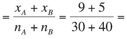0.2

Observed Significance Level: p-value = 2*(0.0351) = 0.0702

Conclusion: Since the test statistic of z = 1.81 falls between the critical bounds of z = ±1.96, we do not reject H₀ with at least 95% confidence. Likewise, since the p-value of 0.0702 is greater than the desired α of 0.05, we do not reject H₀. There is not enough evidence to conclude that the proportion of broken crackers differs for Recipes A and B.

Using Excel to Conduct Analyses of Two Population Means and Variances

Descriptive statistics are needed to conduct the analyses we have done to date: sample means, standard deviations, and counts. If the descriptive statistics are not already given for a set of data, Excel can easily derive the values. In Chapter 4, we referenced the individual functions embedded in Excel for each of the descriptive statistics. Excel also has some programmed capabilities that make the comparatively complex calculations involving the analysis of two or more populations much easier. We can access them through the toolbar in the Data ribbon under the specific button for Data Analysis. If your computer does not show the Data Analysis capability, you can update the application by going to the Windows button and installing the toolkit over the web for later versions of Excel.

Using the Data Analysis toolkit, we can access several powerful programmed functions. Of interest to us in this chapter are the following:

• Descriptive Statistics
• F-Test Two Sample for Variances
• t-Test: Assuming Equal Variances
• t-Test: Assuming Unequal Variances
• t-Test: Paired Two Sample for Means
• z-Test: Two Sample for Means

All of these imbedded programs require the actual data list from each sample, as opposed to summary statistics from each sample. A brief description of each follows.

Descriptive Statistics

To access this Excel program, activate the Data Analysis toolkit on the spreadsheet with the data list and select this program. Enter the range of the data for which you want summary statistics. If a label for the data list heads the column or row of data, include the label and check the box confirming the label is in the first row or column, depending on the orientation of your data. Toward the bottom of the window, click “Summary Statistics.” Click the output range and activate the field by clicking your mouse in that field. Identify a single cell where the beginning of the output should be placed on your spreadsheet. Click “OK” at the top of the box. Output will include, among others, the mean, the standard deviation, the variance, and the count. It is always wise to double check that the count in the output matches the count of values you know to be included in the data list to verify you included the entire list.

F-Test: Two Sample for Variances

To access this Excel program, activate the Data Analysis toolkit on the spreadsheet with the data list and select this program. Enter the range of the data you want for the numerator variable as Variable 1 and the data you want for the denominator variable as Variable 2. If a label for the data list heads the column or row of data, include the label and check the box confirming the label is in the first row or column, depending on the orientation of your data. Since the F-test for the equality of two variances is a two-tailed test, report as the value in the field labeled “Alpha.” Click the output range and activate the field by clicking your mouse in that field. Identify a single cell where the beginning of the output should be placed on your spreadsheet. Click “OK” at the top of the box. Output will include means, variances, counts, df, the calculated test statistic, the one-tailed p-value, and the upper critical bound. Don’t forget that you need to double the reported one-tailed p-value to get the full two-tailed p-value.

t-Test: Assuming Equal Variances

To access this Excel program, activate the Data Analysis toolkit on the spreadsheet with the data list and select this program. Enter the range of the data you want for the first variable as Variable 1 and the data you want for the second variable, which is shown as subtracted from Variable 1 in H₀, as Variable 2. If a label for the data list heads the column or row of data, include the label and check the box confirming the label is in the first row or column, depending on the orientation of your data. Enter the full α shown in the hypothesis test in the field labeled “Alpha.” Click the output range and activate the field by clicking your mouse in that field. Identify a single cell where the beginning of the output should be placed on your spreadsheet. Click “OK” at the top of the box. Output will include means, variances, counts, pooled variance, df, the calculated test statistic, the one-tailed and two-tailed p-values, and the upper critical bound for both a one-tailed and a two-tailed hypothesis test. If your test has a lower-tail rejection region, you need to take the negative of the upper critical bound to find the lower critical bound that is the boundary value for the rejection region.

t-Test: Assuming Unequal Variances

To access this Excel program, activate the Data Analysis toolkit on the spreadsheet with the data list and select this program. Enter the range of the data you want for the first variable as Variable 1 and the data you want for the second variable, which is shown as subtracted from Variable 1 in H₀, as Variable 2. If a label for the data list heads the column or row of data, include the label and check the box confirming the label is in the first row or column, depending on the orientation of your data. Enter the full α shown in the hypothesis test in the field labeled “Alpha.” Click the output range and activate the field by clicking your mouse in that field. Identify a single cell where the beginning of the output should be placed on your spreadsheet. Click “OK” at the top of the box. Output will include means, variances, counts, df, the calculated test statistic, the one-tailed and two-tailed p-values, and the upper critical bound for both a one-tailed and a two-tailed hypothesis test. If your test has a lower-tail rejection region, you need to take the negative of the upper critical bound to find the lower critical bound that is the boundary value for the rejection region.

t-Test: Paired Two Sample for Means

To access this Excel program, activate the Data Analysis toolkit on the spreadsheet with the data list and select this program. Enter the range of the data you want for the first variable as Variable 1 and the data you want for the second variable, which is shown as subtracted from Variable 1 in H₀, as Variable 2. If a label for the data list heads the column or row of data, include the label and check the box confirming the label is in the first row or column, depending on the orientation of your data. Enter the full α shown in the hypothesis test in the field labeled “Alpha.” Click the output range and activate the field by clicking your mouse in that field. Identify a single cell where the beginning of the output should be placed on your spreadsheet. Click “OK” at the top of the box. Output will include means, variances, counts, df, the calculated test statistic, the one-tailed and two-tailed p-values, and the upper critical bound for both a one-tailed and a two-tailed hypothesis test. If your test has a lower-tail rejection region, you need to take the negative of the upper critical bound to find the lower critical bound that is the boundary value for the rejection region.

z-Test: Two Sample for Means

To access this Excel program, activate the Data Analysis toolkit on the spreadsheet with the data list and select this program. Enter the range of the data you want for the first variable as Variable 1 and the data you want for the second variable, which is shown as subtracted from Variable 1 in H₀, as Variable 2. If a label for the data list heads the column or row of data, include the label and check the box confirming the label is in the first row or column, depending on the orientation of your data. Enter the values for each of the known variances. Enter the full α shown in the hypothesis test in the field labeled “Alpha.” Click the output range and activate the field by clicking your mouse in that field. Identify a single cell where the beginning of the output should be placed on your spreadsheet. Click “OK” at the top of the box. Output will include means, variances, counts, df, the calculated test statistic, the one-tailed and two-tailed p-values, and the upper critical bound for both a one-tailed and a two-tailed hypothesis test. If your test has a lower-tail rejection region, you need to take the negative of the upper critical bound to find the lower critical bound that is the boundary value for the rejection region.

Confidence Intervals on the Difference of Means From Two Populations, Independent Samples

Rather than test whether two population means differ, we may want to estimate how different the two means are. When samples are taken randomly from two normally distributed populations with equal variances, the sampling distribution of their difference follows a t-distribution with n₁ + n₂ − 2 degrees of freedom. So, 100(1 − α)% of the samples taken will have a difference that falls within the interval defined by the sample statistic ± the standard error of the sample statistic. When we estimate the difference between two means taken from populations with approximately equal variances, the confidence interval is found with the equation where the pooled variance, s²_p, is defined by the equation we introduced early in this chapter, .

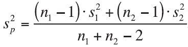Example 5.7.

Holiday shopping accounts for a significant portion of retail sales in the United States. A random sample of 35 households was examined to determine last year’s holiday spending. An earlier random sample of 37 households was similarly examined for the prior year. The results are summarized in the following table. Assuming the populations are approximately normally distributed, use a 95% confidence level to determine the upper and lower bounds on the difference in average household holiday spending between the two years.

Answer

Because the populations are approximately normally distributed and the sample sizes sufficiently large, we will use a t-confidence interval to establish bounds on the difference in average household holiday spending between the two years. To be 95% confident, the 5% risk we are wrong is split between the upper and lower tails of the distribution. The appropriate t-coefficient is t = ±1.994.

Pooled variance estimate:

Upper bound:

Lower bound:

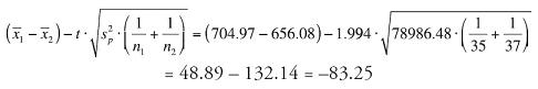
Interpretation: Approximately 95% of the time we take samples of 35 and 37 households from the two years under study, we will find a difference in their average household holiday spending of between −$83.25 and $181.03. Since zero is in the calculated interval, we cannot be certain with 95% confidence that there is any real difference in the average household holiday spending between the two years.

Confidence Intervals on the Difference of Proportions From Two Populations

When sample sizes are sufficiently large, the sampling distribution of the difference in their proportions follows the z-distribution. So, 100(1 − α)% of the samples taken will have a difference that falls within the interval defined by the sample statistic ± the standard error of the sample statistic.

When we estimate the difference between two proportions, the confidence interval is found with the equation

In calculating the standard error for the confidence interval on the difference of two proportions, note that we do not use the pooled estimate of the population proportion, _pooled, as we did in calculating the standard error for the test statistic used in the hypothesis test. We do not use the pooled estimate of the population proportion here because we have not assumed the two population proportions are equal as we did in the null hypothesis of the hypothesis test.

Example 5.8.

Employee sick leave rates are monitored at two manufacturing sites, one located in Denver, Colorado and the other in Kansas City, Missouri. A random sample of 80 Denver employees noted 8 had called in sick for one or more days in the first quarter of the year. In comparison, a random sample of 100 Kansas City employees found 6 had called in sick one or more days in the first quarter of operation there. Use a 95% confidence level to determine the upper and lower bounds on the difference in the proportion of employees calling in sick at the two plants.

Answer

Because the numbers of employees utilizing sick leave are both greater than 5, the samples are sufficiently large to calculate a z-confidence interval on the difference of the two proportions.

= 0.04 ± 0.08055

Lower bound = −0.04055, Upper bound = 0.12055

Interpretation: Approximately 95% of the time we take samples of 80 and 100 employees from the two manufacturing sites, we will find a difference in their employee sick leave rates of between −4.1% and 12.1%. Since zero is in the calculated interval, we cannot be certain with 95% confidence that there is any real difference in the employee sick leave rates at the two sites.