
Testing Proportions From Two or More Populations
As we have seen in earlier chapters, statistical inference involves a claim about some unknown population characteristic, like the population mean. The techniques used have relied on assumptions about the population the sample data were drawn from. Those techniques are said to be parametric in that they measure the degree to which sample data reflect the assumed population parameter (for example, μ for a test of population means). In contrast, chi-square (χ2) analysis examines hypotheses about some property of the distribution being sampled. Chi-square analysis is an example of a set of techniques that are said to be nonparametric because they require fewer assumptions about the nature of the population the data were sampled from. In this chapter, we will discuss the chi-square goodness-of-fit test and the test of independence.
Chi-Square Goodness-of-Fit Tests
Chi-square goodness-of-fit tests involve a multinomial distribution—that is, a set of data that represents multiple outcomes within a single population. A multinomial distribution is used to characterize the probabilities that sampled elements fall into their respective classes of a categorical variable. While the goodness-of-fit test can be applied to a population with two outcomes, its strength is shown when applied to a multinomial distribution with three or more outcomes. Consistent with principles set out in our first chapter, multinomial classes must be mutually exclusive and exhaustive. In addition, the probabilities of the multiple outcomes must remain constant trial to trial, and the trials themselves must be independent.
Unlike previous hypothesis tests of population parameters where the null hypothesis contains the opposite of what you really want to be true, the null hypothesis of the chi-square goodness-of-fit test is a constructive statement about the distribution from which the sample could have been taken. In parametric techniques (for the t-, z-, and F-distributions), the alternative hypothesis contains the real motivation for conducting the test. In the goodness-of-fit test, however, the reason for conducting the test is incorporated into the null hypothesis. For the pragmatic analyst conducting a goodness-of-fit test, good news occurs when the null hypothesis cannot be rejected, for the analysis has shown that the sample data do not differ significantly from the distribution specified in the null hypothesis. When the analyst fails to reject the null hypothesis in the goodness-of-fit test, the results present some evidence that the distribution proposed in the null hypothesis can be considered a plausible model for later analysis and forecasting.
The multinomial experiment underlying the goodness-of-fit test requires the sample size to be sufficiently large so that the expected frequencies for each class based on the hypothesized distribution will be at least five. In the event a class has an expected frequency less than five, the analyst should collapse the probability and expected frequency of that class with those of a neighboring class.
Forming hypotheses is the first step of any analytic project. The goodness-of-fit test begins with a hypothesis about the distribution the sample data could have been drawn from.
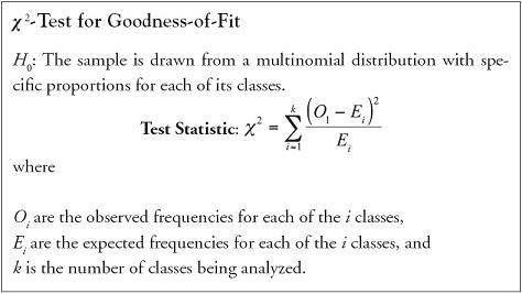
- H0: The sample is drawn from a multinomial distribution with specific proportions for each of its classes.
- H1: The sample is not drawn from a multinomial distribution with specific proportions for each of its classes.
Let’s investigate several scenarios.
Scenario 1: According to the 2009 DuPont Global Automotive Color Popularity Report, automotive color rankings worldwide place silver first with 25% of the global market, black second with 23%, white third with 16%, gray fourth with 13%, blue fifth with 9%, and red sixth with 8%. All other car colors make up the remaining 6% of the market. The appropriate null and alternative hypotheses are
- H0: pSilver = 0.25, pBlack = 0.23, pWhite = 0.16, pGray = 0.13, pBlue = 0.09, pRed = 0.08, pOther = 0.06
- H1: At least one of the proportions differs from the stated value.
In this scenario, proportions for each of the possible outcomes are known and add to 1. (Scenario taken from http://www2.dupont.com/Automotive/en_US/news_events/article20091201.html.)
Scenario 2: A county ambulance service provider wants to test whether calls for ambulances are equally distributed over the days of the week. The appropriate null and alternative hypotheses are
- H0: pM = pTu = pW = pTh = pF = pF = pSat = pSun =

- H1: At least one of the proportions differs from the stated value.
In this scenario, proportions for each of the possible outcomes are assumed to be equal and add to 1.
Scenario 3: A random sample of average grocery expenses for 350 people living in Mannville indicated the sample mean was $35.34 with a sample standard deviation of $4.15. Could the sample have been drawn from a normal population with a population mean of $36 per person? The appropriate null and alternative hypotheses are
- H0: The sample is from a population of average grocery expenses that are normally distributed around a population mean of $36.
- H1: The sample is not from a population of average grocery expenses that are normally distributed around a population mean of $36.
Note that the distribution in Scenario 3 considers a continuous, quantitative variable. However, by breaking the range of the distribution into segments, we can consider the likelihood that one person’s grocery expense falls into any segment and treat the set of expenditure segments as a categorical variable.
In all three scenarios, the null hypothesis contains a constructive statement about the distribution from which the sample could have been taken and against which the sample data will be tested.
The frequency we should expect for each class, Ei, is the expected proportion for each class times the overall sample size, n. Because the null hypothesis is assumed true, the expected values are derived from the null hypothesis. The squared differences between the observed sample frequencies and the expected frequencies are compared to the expected frequencies for each class as a measure of how closely the sample data reflect the hypothesized distribution and form the basis of the test statistic.
The chi-square distribution is a family of distributions that is highly skewed for small degrees of freedom but approaches the normal distribution for large degrees of freedom.
The degrees of freedom for the chi-square distribution are dependent on the number of population parameters being estimated. In Scenarios 1 and 2, there are no population parameters estimated, so the degrees of freedom in each are simply one less than the number of classes in the multinomial distribution. The degrees of freedom for Scenarios 1 and 2 are 7 − 1 = 6. In Scenario 3, the null hypothesis specifies the population mean is $36, but it does not specify the value of the population standard deviation. For Scenario 3, the degrees of freedom are one less than the number of classes minus one because we are estimating the population standard deviation. The degrees of freedom for Scenario 3 are k − 2, where k is the number of categories in the frequency distribution.
Example 7.1.
Historic performance records for an electronic component indicate that 92% have no evidence of flawed function, 5% show evidence of one flaw, and 3% registered two or more flaws during testing. A sample of 200 components selected from the current batch indicates 179 have no flaws, 12 have one flaw, and 9 have two or more flaws. Is there sufficient reason at the 0.05 level of significance to conclude the current batch has a different performance profile than is historically established?
Answer
H0: p0 = 0.92, p1 = 0.05, p2+ = 0.03
Current performance data mirror the historic performance profile for the component.
H1: At least one proportion differs from the performance profile for this component.
At least one of the proportions for performance categories differs from those for the historic performance profile.
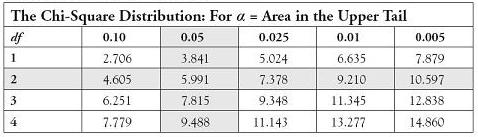
Decision Rule: For df = 3 − 1 = 2 and α = 0.05, we will reject the null hypothesis if the calculated test statistic falls above χ2 = 5.991. See Table 7.1 below.
Table 7.1. Using the Chi-Square Distribution to Find the Appropriate Critical Bound for df = 2 and α = 0.05
Test Statistic:
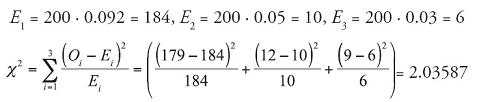
Observed Significance Level: Using Excel’s built-in function =chidist and 2 degrees of freedom, we find that the p-value = 0.36134.
Conclusion: Since the test statistic of χ2 = 2.036 falls below the critical bound of 5.991, we do not reject H0 with at least 95% confidence. Likewise, since the p-value of 0.36 is much greater than the desired α of 0.05, we do not reject H0. There is not enough evidence to conclude current performance data differ from the historic performance profile for the component. If this were a set of criteria to determine salability, the current batch of components could be shipped to the vendor.
An important application of the goodness-of-fit test is the test for normality. It is a complex procedure, but worthy of developing an example to discuss.
Example 7.2.
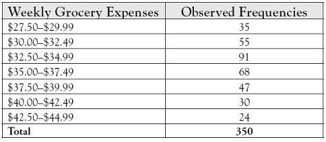
According to a regional study, the average weekly grocery expense in an area in 2010 was $36 per person. The results of a random sample of 350 people living in Mannville are shown in Table 7.2. Could the sample have been drawn from a normal population with a population mean of $36 per person? Use a 99% level of confidence.
Table 7.2. Observed Frequencies for Weekly Grocery Expenses
Answer
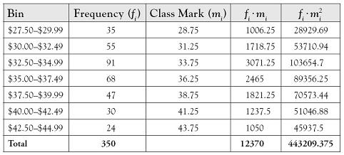
Some work needs to be done before the formal hypothesis test is conducted. First we need to compute the standard deviation for the sample using the estimation procedures we presented in Chapter 2.
Table 7.3. Computational Table to Support Estimate of Standard Deviation
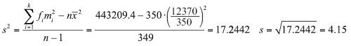
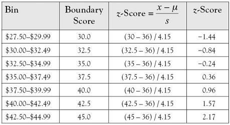
We use the calculated standard deviation to compute the z-score that corresponds to each of the bin boundaries, and, from the z-scores, compute the amount of area that occurs under the standard normal curve between subsequent pairs of z-scores. Note that we are using the hypothesized value of the population mean, μ, in the calculation of the z-score, not the sample mean, ![]() , because the question posed whether the data could have come from a normal population with a mean of $36.
, because the question posed whether the data could have come from a normal population with a mean of $36.
Table 7.4. Computation of z-Scores for Bin Boundaries
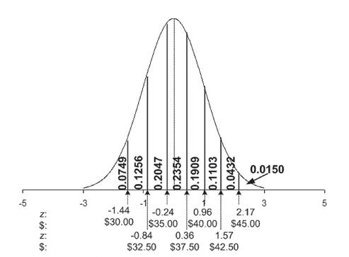
The area in the left tail is simply found on the z-table as the amount of area below a z-score of −1.44. The area of the second region is found by taking the area below a z-score of −0.84, which is 0.2005 and then subtracting the area to the left of its lower bound, which yields 0.1254, and so on, across each region of the distribution.
Once we know the probability of each region, we use those probabilities to compute the expected frequency for each bin by multiplying the probability times the 350 people sampled.
Table 7.5. Computation of Expected Values for Key Regions

Figure 7.1. Normal Distribution Showing Areas for Key Regions
We are now ready to begin the hypothesis test.
H0: The sample is from a population of average grocery expenses that are normally distributed around a population mean of $36.
H1: The sample is not from a population of average grocery expenses that are normally distributed around a population mean of $36.
Decision Rule: The null hypothesis contains the assumption that μ = 36, but there is no assumption about the value of the standard deviation. So our degrees of freedom must be reduced by an additional degree. For df = k − 2 = 8 − 2 = 6 and α = 0.01, the critical bound of the rejection region is χ2 = 16.812. We will reject the null hypothesis if the test statistic is greater than 16.812.
Test Statistic:
Table 7.6. Computation of Chi-Square Test Statistic
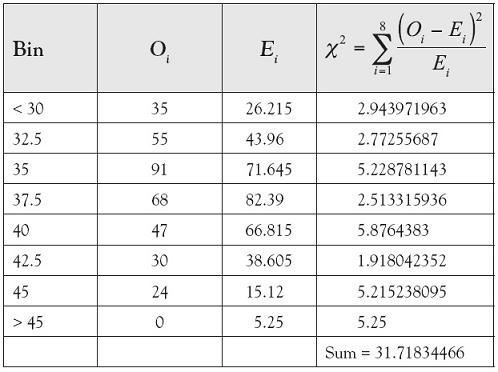
χ2 = 31.718
Observed Significance Level: Using Excel’s built-in function =chidist and 6 degrees of freedom, we find the p-value = 1.848 × 10⁻⁵.
Conclusion: Since the test statistic of χ2 = 31.718 falls above the critical bound of 16.812, we reject H0 with at least 99% confidence. Likewise, since the p-value of 1.848 × 10⁻⁵ is much smaller than the desired α of 0.01, we reject H0. There is sufficient evidence to conclude that the sample of 350 weekly grocery expenses could not have come from a normal distribution with a mean of $36.
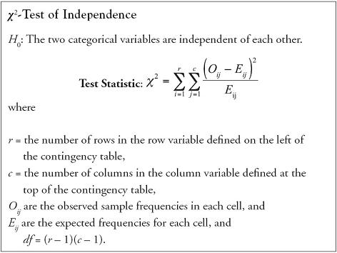
Tests of Independence
The independence of two qualitative variables can be determined using the chi-square test, provided the two variables are each parsed into two or more subcategories. The chi-square test of independence can be used analyzing data involving two categorical variables, where the data are arranged in a grid of r rows and c columns called a contingency table.
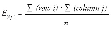
By assuming the two variables are independent of one another, we can use the chi-square statistic to measure how much difference there is between actual and expected counts in each of the classes. But how does that work? When two events are independent, the fact that one event occurs does not influence the probability that the other event also occurs. So the joint probability of the two events occurring is the simple probability that one event occurs times the simple probability the other event occurs. In a contingency table, that means that the joint probability a sampled element is in a given row and column equals the simple probability the element is in a given row times the simple probability it is also in that particular column. Each of those simple probabilities is the total number of sampled elements in that row or column divided by the number of elements sampled. Under the assumption of independence between the row variable and the column variable, the following is true:

To compute the chi-square test statistic, we need the expected value. That is the product of the joint probability times the number of elements sampled.
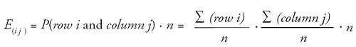
The computational shortcut, then is to cancel one factor of n from the numerator and one from the denominator on the right side of the equation, which means the expected value for each cell is computed by multiplying the sum of elements in that cell’s row times the sum of elements in that cell’s column divided by the total number of elements sampled.
Example 7.3.
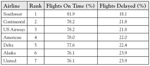
The Bureau of Transportation Statistics tracks and reports on-time performance for major commercial airline carriers in the United States. The top seven airline carriers ranked on overall percentage of reported flight operations arriving on time for operations 09/1987 through 10/2010 are shown in Table 7.7.
Table 7.7. U.S. Flight Operations, 9/1987 Through 10/2010
Answer
Assuming samples of 1000 flights per airline, use the 0.05 level of significance to determine whether being on time is independent of individual airlines.
H0: Being on time is independent of individual airlines.
H1: Being on time is dependent on individual airlines.
Decision Rule: For df = (r − 1)(c − 1) = (7 − 1)(2 − 1) = 6 and α = 0.05, we will reject the null hypothesis if the calculated test statistic falls above χ2 = 12.592.
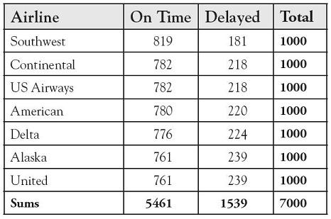
Test Statistic: For 1000 flights per airline, the observed frequencies are shown in Table 7.8.
Table 7.8. Calculation of the Observed Frequencies per 1000 Flights
To compute the expected values, use Table 7.9.
Table 7.9. Calculation of Expected Values per 1000 Flights

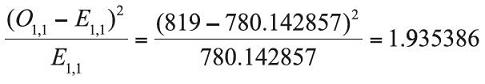
To review how each cell’s contribution to the chi-square test statistic is formed, we include detail of the calculation for Southwest’s on-time flights, the first row and the first column of the data:
 as shown in Table 7.10
The contributions toward the test statistic are shown in Table 7.10.
Table 7.10. Calculation of the Chi-Square Test Statistic

χ2 = 13.216
Observed Significance Level: Using Excel’s built-in function =chidist and 6 degrees of freedom, we find the p-value = 0.0397.
Conclusion: Since the test statistic of χ2 = 13.216 falls above the critical bound of 12.592, we reject H0 with at least 95% confidence. Likewise, since the p-value of 0.0397 is less than the desired α of 0.05, we reject H0. There is enough evidence to conclude that the on-time performance of airline flights is dependent on individual airlines. Said another way, there is evidence to conclude that the percent of on-time flights differs across the top seven major U.S. commercial airlines. (Example taken from http://airconsumer.ost.dot.gov/reports/2010/December/2010DecemberATCR.DOC.)