Chapter 8

An Introduction to Regression Analysis

Until this point, with the exception of covariance and correlation coefficient, the focus has been on a single variable. However, there are few, if any, economic phenomena that can be analyzed solely using its own information. Even in the simplest economic issues such as quantity demanded, there are at least two variables, a quantity and a price. Furthermore, many economic affairs are too complicated to be analyzed and explained fully by merely observing the matter by itself without any consideration to other economics, social, cultural, and political factors that usually affect most economic problems. For example, it does not suffice to analyze data on income in order to determine or forecast future incomes. Such a study does not provide a reasonable estimate of the current situation, let alone future forecasts. Let us explore, briefly, what other factors might affect income. First, we have to decide whether the orientation of the study is macro or microeconomics. At the microeconomics level the focus on income can be personal income or family income. For an individual, income is zero for many years. During these years the individual is growing up and attending school. In other words, he or she is acquiring human capital, which will affect earned income when the individual secures a job. Other factors include one’s natural ability, talent, work ethic, exertion, years of experience, and seniority, to name a few. There are some other factors that, at least in theory, should not have an effect on one’s income, but in reality they do, such as gender and race. At the macroeconomics level the determinants of income, which in this case should be referred to as the national income, are functions of the nation’s productivity, its resources, population size, education levels, economic cycles, seasonal cycles, and other factors.

There are many powerful tools in statistical analysis that permit incorporating the factors that determine a phenomenon such as income. One such tool is regression analysis. The regression methodology acknowledges that most real life occurrences are subject to random error. Take, for example, the income of a person. It is easy to calculate the average income of the nation. Let us take a single person and compare his or her income to the average. Chances are that the income of the person is not going to be the same as the national average. One can argue that it would be unreasonable to expect the income of a person chosen at random to be the same as the average income of the nation because the person is likely to have a different level of education, years of experience, talent, ambition, health, and so forth than the average person. All of these do affect income. The important thing is that even if we account for all reasonable sources of differences between two people, there still will be a difference in income due to random factors beyond our control, recognition, or ability to measure them. The presence of difference between observations is nothing new, and we addressed that when we discussed the concept of individual error and error in general throughout this text. In the case of comparing a person to the average, most of the difference can be attributed to the differences in the influencing factors such as education, experience, and talent. In regression analysis, we try to account for these sources of influence and “explain” part of the error. Recall that a basic definition of error in statistics is “whatever that cannot be explained.” So the deviation of one person’s income from the average income is called individual error. In statistics it makes more sense to talk about averages because of the existence of random error. Averaging things removes the random error, which by definition has an expected value or an average equal to zero. In Chapter 2, we introduced variance, which gives a measure of error. In the same chapter we discussed standard deviation, which is the average error. In regression analysis we explain the part of the error that is caused by differences in the factors that affect the phenomenon of interest, in this case the income. After accounting for the role of all the influencing factors that determine income, there is a random component that remains unexplainable, which by definition becomes the new “error.”1 Briefly, the regression analysis is designed to minimize the squares of errors of observations from a hypothetical line that provides a relationship between a dependent variable, such as income, and an independent variable such as education. Note that errors are simply deviations of observations from the expected value. In descriptive statistics the expected value is simply the mean. In regression analysis, the regression line is the expected value.

We can extend the simple regression analysis from the case of one variable to as many variables as deemed necessary. As the number of explanatory variables increases, the regression model should be able to explain more of the deviations in the dependent variable, which in our example is the income. This statement is valid only if we have the correct determining factors, are also called independent variables and, all the appropriate independent variables are included without having irrelevant variables in the model. In the above example, the independent variables are education, years of experience, talent, ambition, and so forth. As mentioned earlier, there are factors that influence the dependent variable even though they should not, such as gender and race, and factors that influence income but cannot be controlled or anticipated by the model, such as a war, natural disaster, and so on. We include these variables in the models as control variables. Control variables such as war or natural disaster have good economic explanations. They are the variables that are assumed constant under the ceteris paribus assumption of economic theory.

The simple regression model consists of one dependent variable and one independent variable plus an error term.

Income = β0 + β1 Education + ε(8.1)

where, income is the dependent variable,

education is the independent variable,

β0 is the intercept,

β1 is the slope, and

ε is the error term.

This chapter is a brief introduction to a vast topic.2 The independent variable is believed to be outside of the model and is not to be explained in any manner. Here we are not interested in why people obtain the level of education they do. Instead we are observing one’s educational level and use it to explain his or her income. The dependent variable is endogenous to the model, which means the model is used to estimate the value of the dependent variable based on the level of income. In other words, the model determines the income, given a specific value of education. The Greek letters β0 and β1 are the parameters of the model. They are also called the intercept and the slope, respectively. The interpretation of β1 is that for every unit change in education, income will change by the magnitude of β1 and in the direction of its sign. The intercept β0 provides an estimate of income when one has zero education. Finally, ε the error term, accounts for everything else that affects income, other than education, plus the random error inherent in real phenomena.

This simplistic model explains income with one variable. The hypothesized claim for the slope of the regression line, β1, is that it is expected to be positive. This claim is based on theory and common sense. One expects higher income with more education, since education is a kind of investment called human capital. An educated person is more knowledgeable and hence, more productive, and thus deserves higher income per unit of time than someone with less education, other things equal. There are several advantages to using regression analysis. One of the more important ones is the fact that not only can we measure the contribution of the determinants of a dependent variable such as income, but we can also test to see if the determinants are actually significant. A typical inference about a regression model consists of two different tests. The one that tests the overall significance of the model is based on the F test. In this case, the amount of the variation in the dependent variable that is explained by the model is compared to the amount that still remains unexplained. The portion that is explained by the model is called mean squared regression (MSR). Recall that the sum of squares of the portions not explained, divided by appropriate degrees of freedom is the same as variance, which in the jargon of regression analysis is called mean squared error (MSE). In Chapter 4, we explained that the variance has a chi-squared distribution. The MSR also has a chi-squared distribution since it has similar distributional properties as a variance. Theorem 4.5 from Chapter 4 states that the ratio of two chi-squared distribution functions follows an F distribution. Therefore, we can use an F statistics to test the relative magnitude of the portion of the variation in the dependent variable that is explained by the model to the portion that is not. The null and alternative hypotheses for the model are:

H0: Model is not good    H1: Model is good

The testing procedure is the same as before. If the p value is small enough, reject the null hypothesis; otherwise, fail to reject it. Once the above null hypothesis is rejected, then the individual slopes are tested for significance. The customary null hypothesis is that the slope of interest is zero. When a slope is zero it indicates that the corresponding variable does not have any explanatory power, and it does not contribute to the reduction of the variations in the error.

H0: βEducation = 0    H1: βEducation > 0

The appropriate test statistics for this hypothesis is a t statistics. Testing procedure is the same as usual. Reject the null hypothesis if the corresponding p value is low enough. All software designed to perform statistical analysis can perform regression analysis with a relatively easy set of commands or procedures, or both. In fact, many of the commercially available software are menu-driven, similar to a typical application software. Most have reasonably good help features that will show the necessary steps or commands. Even Microsoft Excel, a spreadsheet software, has a menu driven procedure to perform regression analysis, to provide test statistics for testing the model and slopes, and to provide estimates of slopes and the explanatory power of the model.3

Example 8.1

Let us test the hypothesis that education increases income. As pointed out earlier, there are numerous measures of income, from per capita personal income to the national income; the former represented a microeconomics aspect of income, while the latter is a macroeconomics perspective.4 Care must be taken to analyze the data in light of its nature and not to imply or indicate more than the meaning of the outcome. The data is presented in Table 8.1.

Table 8.1. Data on Education and Income from 1970 to 2010 for the United States

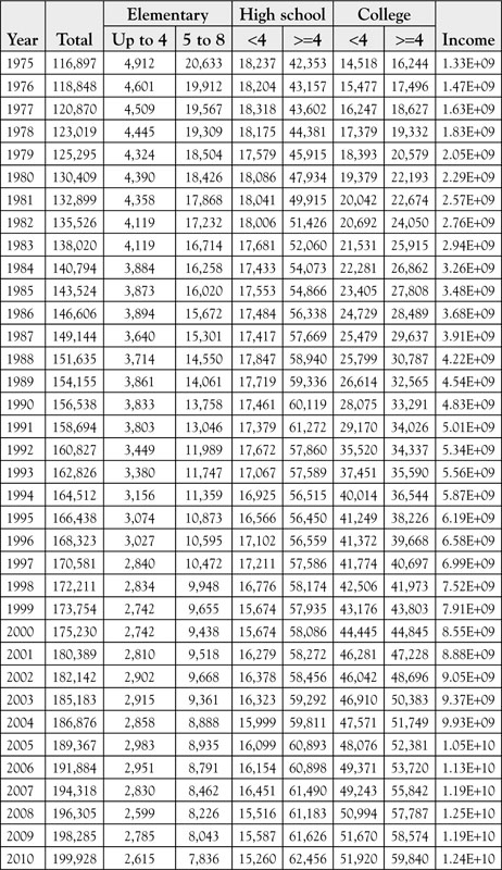
First, we regress income on the total number of people in the United States with education, regardless of the level of education.5 See Table 8.2. The regression output is obtained from Excel. We will focus on the row named “Total,” which refers to the name we used for the independent variable representing education. Remember that the data for education are represented in thousands of people. The coefficient for the independent variable is 127,095.6414. Therefore, for every 1,000 people who are educated, the income increases by $127,095. The other information in the output indicates that the model is a good model.

Next, let us regress the income on the number of people with four or more years of college (see Table 8.3).

The coefficient for the independent variable “4 or more years of college education” is $253,879. This indicates that for every 1,000 persons obtaining four or more years of college education, income increases by $253,879. This figure is twice the $127,095 we obtained for overall increase in education attainment. Therefore, as expected, more education results in higher income for the country.

What do you think would happen if we regressed income on the number of people with less than 4 years of education? The average number of years of education in the United States is much higher than 4 years of education. A person with such a low educational level will cause a reduction in the expected income of the country. Let us see if the regression analysis can demonstrate this point. The result of regressing income on up to 4 years of elementary education is shown in Table 8.4.

As anticipated, the coefficient of the independent variable is negative, indicating that for every 1,000 people who are over 25 years of age the income declines by $3,751,795. Other statistics in the table indicate that the model is a good model. It is important to caution the reader that these models are very simplistic, and there are more issues that have to be addressed. A comprehensive study of the impact on education is a huge undertaking, and this brief introduction is not sufficient to identify the true impact of education on income. One shortcoming of these examples is that they do not consider other factors that affect income, as discussed earlier. The simple regression analysis is easily extended to include all the variables that a researcher deems necessary. The main determining factor for including a variable in a regression model is the theory in the discipline in which the research is conducted. In our case, the governing theory belongs to the field of economics.

Income = β0 + β1 Education + β2 Experience
+ β3 Race + β4 Gender + β5 Determination + ε(8.2)

The previous model is a typical model based on the variables we identified earlier as important. Note that the list is not exhaustive. One reason is that social variables are somewhat correlated. Education is not really independent of race or gender. Although there is no justifiable reason for education to be influenced by race or gender, the reality in the United States is that it is. Similarly, there is no reason to include race and gender as control variables in the model explaining the determinants of income. However, the fact is that in the current US society these variables do affect the level of income, other things equal. The second reason for limiting the number of variables is that, usually few important variables are sufficient to provide reasonable estimates or forecasts of the dependent variable. Generally, if two models are performing about the same, the one with fewer variables is preferred. One variable merits additional comments. The variable is “determination.” There is no doubt that the amount of effort that a person puts into his or her job does affect the resulting income. Thus, the hypothesized value of β5 is positive. However, there is no acceptable way of measuring one’s resolve or how much effort one puts into his or her job. It is fairly easy to identify those that slack off or those that exert themselves, but neither can be measured. More importantly, any arbitrary ranking or measurement of “determination” is inaccurate and incomplete in the sense that it cannot be compared because it is a not a cardinal measure. Frequently, we face this problem in economics. For example, there is no cardinal measure of utility, which is a very important economic concept. The discussion of how we deal with the inability to measure utility with cardinal measures is beyond the scope of this text. In the case of variables such as “determination” in regression model, we have two alternatives. The first one is to accept that it is not a measurable phenomenon and not worry about including it in the model. The consequence is that the error term is enlarged, and there will be more of the variation in the dependent variable that cannot be explained as compared to the case if we could measure “determination” and use it in the model. This exclusion has serious consequences and is usually covered under misspecification of the model. The second method is to use a proxy variable that could represent the desired variable, albeit, not precisely or accurately. Can you think of a good proxy for “determination”?

A typical way of writing a model with unknown number of variables is of the form:

Y = β0 + β1X1 + β2X2 + … + βK XK + ε(8.3)

Each beta represents the contribution of the corresponding factor to an explanation of the dependent variable, keeping all the other factors constant.

Regression analysis is a powerful and useful tool used in many areas of science but has a special place in economics. As one might expect, there are many issues that pertain to economic reality that need not be applicable to other areas of science. We have already seen two such cases. One is the fact that the independent variables are somewhat related to each other in economics. This is due to the fact that many, if not all economic factors are subject to the economics and social realities of the same country. The same applies to the individual firms and people in a country. In many other fields, it is much easier to ensure that exogenous variables are independent from each other, which is a requirement of regression analysis.6 The second issue is the role of factors that are social in nature and reflect the social/cultural structure of a country. For example, the fact is that race and gender influence one’s income. There is no theoretical reason for such a role, except racism and chauvinism. Consequently, a special branch of science has been created called econometrics.