Example of Bivariate Analysis
This example uses the SAT.jmp sample data table. SAT test scores for students in the 50 U.S. states, plus the District of Columbia, are divided into two areas: verbal and math. You want to find out how the percentage of students taking the SAT tests is related to verbal test scores for 2004.
1. Open the SAT.jmp sample data table.
2. Select Analyze > Fit Y by X.
3. Select 2004 Verbal and click Y, Response.
4. Select % Taking (2004) and click X, Factor.
5. Click OK.
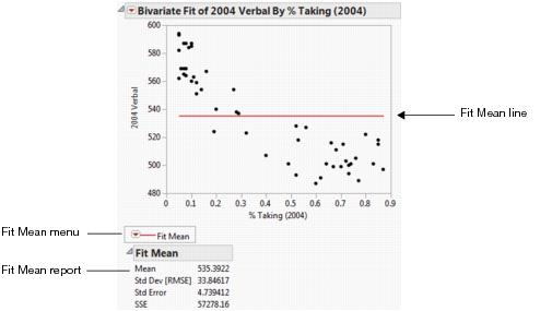
Figure 5.2 Example of SAT Scores by Percent Taking
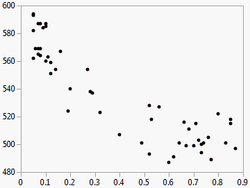
You can see that the verbal scores were higher when a smaller percentage of the population took the test.
Launch the Bivariate Platform
You can perform a bivariate analysis using either the Fit Y by X platform or the Bivariate platform. The two approaches give equivalent results.
• To launch the Fit Y by X platform, select Analyze > Fit Y by X.
or
• To launch the Bivariate platform, from the JMP Starter window, click on the Basic category and click Bivariate.
Figure 5.3 The Bivariate Launch Window
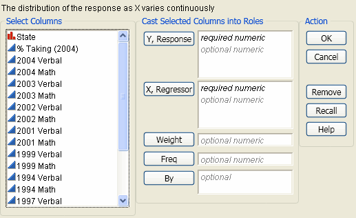
For information about this launch window, see “Introduction to Fit Y by X” chapter.
The Bivariate Plot
To produce the plot shown in Figure 5.4, follow the instructions in “Example of Bivariate Analysis”.
Figure 5.4 The Bivariate Plot
Note: Any rows that are excluded in the data table are also hidden in the Bivariate plot.
The Bivariate report begins with a plot for each pair of X and Y variables. Replace variables in the plot by dragging and dropping a variable, in one of two ways: swap existing variables by dragging and dropping a variable from one axis to the other axis; or, click on a variable in the Columns panel of the associated data table and drag it onto an axis.
You can interact with this plot just as you can with other JMP plots (for example, resizing the plot, highlighting points with the arrow or brush tool, and labeling points). For details about these features, see the Using JMP book.
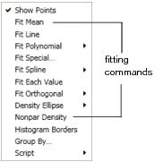
You can fit curves on the plot and view statistical reports and additional menus using the fitting commands that are located within the red triangle menu. See “Fitting Commands and General Options”.
Fitting Commands and General Options
Note: The Fit Group menu appears if you have specified multiple Y variables. Menu options allow you to arrange reports or order them by RSquare. See the Fitting Linear Models book for more information.
The Bivariate Fit red triangle menu contains the fitting commands and general options.
Figure 5.5 Fitting Commands and General Options
|
Show Points
|
Hides or shows the points in the scatterplot. A check mark indicates that points are shown.
|
|
Histogram Borders
|
Attaches histograms to the x- and y-axes of the scatterplot. A check mark indicates that histogram borders are turned on. See “Histogram Borders”.
|
|
Group By
|
Lets you select a classification (or grouping) variable. A separate analysis is computed for each level of the grouping variable, and regression curves or ellipses are overlaid on the scatterplot. See “Group By”.
|
|
Script
|
Contains options that are available to all platforms. These options enable you to redo the analysis or save the JSL commands for the analysis to a window or a file. For more information, see Using JMP.
|
Each fitting command adds the following:
• a line, curve, or distribution to the scatterplot
• a red triangle menu to the report window
• a specific report to the report window
Figure 5.6 Example of the Fit Mean Fitting Command
|
Fit Mean
|
Adds a horizontal line to the scatterplot that represents the mean of the Y response variable.
|
See “Fit Mean”.
|
|
Fit Line
|
Adds straight line fits to your scatterplot using least squares regression.
|
|
|
Fit Polynomial
|
Fits polynomial curves of a certain degree using least squares regression.
|
|
|
Fit Special
|
Transforms Y and X. Transformations include: log, square root, square, reciprocal, and exponential. You can also turn off center polynomials, constrain the intercept and the slope, and fit polynomial models.
|
See “Fit Special”.
|
|
Fit Spline
|
Fits a smoothing spline that varies in smoothness (or flexibility) according to the lambda (λ) value. The λ value is a tuning parameter in the spline formula.
|
See “Fit Spline”.
|
|
Fit Each Value
|
Fits a value to each unique X value, which can be compared to other fitted lines, showing the concept of lack of fit.
|
See “Fit Each Value”.
|
|
Fit Orthogonal
|
Fits lines that adjust for variability in X as well as Y.
|
See “Fit Orthogonal”.
|
|
Density Ellipse
|
Draws an ellipse that contains a specified mass of points.
|
See “Density Ellipse”.
|
|
Nonpar Density
|
Shows patterns in the point density, which is useful when the scatterplot is so darkened by points that it is difficult to distinguish patterns.
|
See “Nonpar Density”.
|
Fitting Command Categories
Fitting command categories include regression fits and density estimation.
|
Category
|
Description
|
Fitting Commands
|
|
Regression Fits
|
Regression methods fit a curve through the points. The curve is an equation (a model) that is estimated using least squares, which minimizes the sum of squared differences from each point to the line (or curve). Regression fits assume that the Y variable is distributed as a random scatter above and below a line of fit.
|
Fit Mean
Fit Line
Fit Polynomial
Fit Special
Fit Spline
Fit Each Value
Fit Orthogonal
|
|
Density Estimation
|
Density estimation fits a bivariate distribution to the points. You can either select a bivariate normal density, characterized by elliptical contours, or a general nonparametric density.
|
Fit Density Ellipse
Nonpar Density
|
Fit the Same Command Multiple Times
You can select the same fitting command multiple times, and each new fit is overlaid on the scatterplot. You can try fits, exclude points and refit, and you can compare them on the same scatterplot.
To apply a fitting command to multiple analyses in your report window, hold down the CTRL key and select a fitting option.
Fit Mean
Using the Fit Mean command, you can add a horizontal line to the scatterplot that represents the mean of the Y response variable. You can start by fitting the mean and then use the mean line as a reference for other fits (such as straight lines, confidence curves, polynomial curves, and so on).
Figure 5.7 Example of Fit Mean
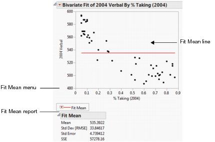
Fit Mean Report
The Fit Mean report shows summary statistics about the fit of the mean.
|
Mean
|
Mean of the response variable. The predicted response when there are no specified effects in the model.
|
|
Std Dev [RMSE]
|
Standard deviation of the response variable. Square root of the mean square error, also called the root mean square error (or RMSE).
|
|
Std Error
|
Standard deviation of the response mean. Calculated by dividing the RMSE by the square root of the number of values.
|
|
SSE
|
Error sum of squares for the simple mean model. Appears as the sum of squares for Error in the analysis of variance tables for each model fit.
|
Fit Line and Fit Polynomial
Using the Fit Line command, you can add straight line fits to your scatterplot using least squares regression. Using the Fit Polynomial command, you can fit polynomial curves of a certain degree using least squares regression.
Figure 5.8 Example of Fit Line and Fit Polynomial
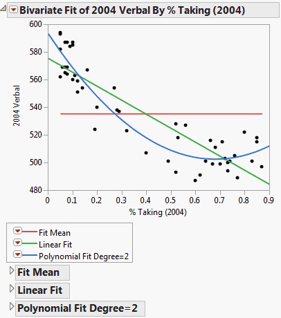
Figure 5.8 shows an example that compares a linear fit to the mean line and to a degree 2 polynomial fit.
Note the following information:
• The Fit Line output is equivalent to a polynomial fit of degree 1.
• The Fit Mean output is equivalent to a polynomial fit of degree 0.
Linear Fit and Polynomial Fit Reports
The Linear Fit and Polynomial Fit reports begin with the equation of fit.
Figure 5.9 Example of Equations of Fit
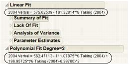
Note: You can edit the equation by clicking on it.
Each Linear and Polynomial Fit Degree report contains at least three reports. A fourth report, Lack of Fit, appears only if there are X replicates in your data.
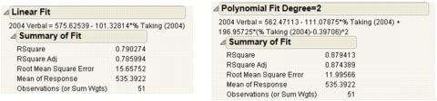
Summary of Fit Report
The Summary of Fit reports show the numeric summaries of the response for the linear fit and polynomial fit of degree 2 for the same data. You can compare multiple Summary of Fit reports to see the improvement of one model over another, indicated by a larger Rsquare value and smaller Root Mean Square Error.
Figure 5.10 Summary of Fit Reports for Linear and Polynomial Fits
|
RSquare
|
Measures the proportion of the variation explained by the model. The remaining variation is not explained by the model and attributed to random error. The Rsquare is 1 if the model fits perfectly.
The Rsquare values in Figure 5.10 indicate that the polynomial fit of degree 2 gives a small improvement over the linear fit.
|
|
RSquare Adj
|
Adjusts the Rsquare value to make it more comparable over models with different numbers of parameters by using the degrees of freedom in its computation.
|
|
Root Mean Square Error
|
Estimates the standard deviation of the random error. It is the square root of the mean square for Error in the Analysis of Variance report. See Figure 5.12.
|
|
Mean of Response
|
Provides the sample mean (arithmetic average) of the response variable. This is the predicted response when no model effects are specified.
|
|
Observations
|
Provides the number of observations used to estimate the fit. If there is a weight variable, this is the sum of the weights.
|
Lack of Fit Report
Note: The Lack of Fit report appears only if there are multiple rows that have the same x value.
Using the Lack of Fit report, you can estimate the error, regardless of whether you have the right form of the model. This occurs when multiple observations occur at the same x value. The error that you measure for these exact replicates is called pure error. This is the portion of the sample error that cannot be explained or predicted no matter what form of model is used. However, a lack of fit test might not be of much use if it has only a few degrees of freedom for it (few replicated x values).
Figure 5.11 Examples of Lack of Fit Reports for Linear and Polynomial Fits
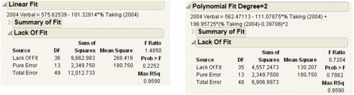
The difference between the residual error from the model and the pure error is called the lack of fit error. The lack of fit error can be significantly greater than the pure error if you have the wrong functional form of the regressor. In that case, you should try a different type of model fit. The Lack of Fit report tests whether the lack of fit error is zero.
|
Source
|
The three sources of variation: Lack of Fit, Pure Error, and Total Error.
|
|
DF
|
The degrees of freedom (DF) for each source of error.
• The Total Error DF is the degrees of freedom found on the Error line of the Analysis of Variance table (shown under the “Analysis of Variance Report”). It is the difference between the Total DF and the Model DF found in that table. The Error DF is partitioned into degrees of freedom for lack of fit and for pure error.
• The Pure Error DF is pooled from each group where there are multiple rows with the same values for each effect. See “Statistical Details for the Lack of Fit Report”.
• The Lack of Fit DF is the difference between the Total Error and Pure Error DF.
|
|
Sum of Squares
|
The sum of squares (SS for short) for each source of error.
• The Total Error SS is the sum of squares found on the Error line of the corresponding Analysis of Variance table, shown under “Analysis of Variance Report”.
• The Pure Error SS is pooled from each group where there are multiple rows with the same value for the x variable. This estimates the portion of the true random error that is not explained by model x effect. See “Statistical Details for the Lack of Fit Report”.
• The Lack of Fit SS is the difference between the Total Error and Pure Error sum of squares. If the lack of fit SS is large, the model might not be appropriate for the data. The F-ratio described below tests whether the variation due to lack of fit is small enough to be accepted as a negligible portion of the pure error.
|
|
Mean Square
|
The sum of squares divided by its associated degrees of freedom. This computation converts the sum of squares to an average (mean square). F-ratios for statistical tests are the ratios of mean squares.
|
|
F Ratio
|
The ratio of mean square for lack of fit to mean square for Pure Error. It tests the hypothesis that the lack of fit error is zero.
|
|
Prob > F
|
The probability of obtaining a greater F-value by chance alone if the variation due to lack of fit variance and the pure error variance are the same. A high p value means that there is not a significant lack of fit.
|
|
Max RSq
|
The maximum R2 that can be achieved by a model using only the variables in the model.
|
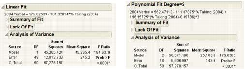
Analysis of Variance Report
Analysis of variance (ANOVA) for a regression partitions the total variation of a sample into components. These components are used to compute an F-ratio that evaluates the effectiveness of the model. If the probability associated with the F-ratio is small, then the model is considered a better statistical fit for the data than the response mean alone.
The Analysis of Variance reports in Figure 5.12 compare a linear fit (Fit Line) and a second degree (Fit Polynomial). Both fits are statistically better from a horizontal line at the mean.
Figure 5.12 Examples of Analysis of Variance Reports for Linear and Polynomial Fits
|
Source
|
The three sources of variation: Model, Error, and C. Total.
|
|
DF
|
The degrees of freedom (DF) for each source of variation:
• A degree of freedom is subtracted from the total number of non missing values (N) for each parameter estimate used in the computation. The computation of the total sample variation uses an estimate of the mean. Therefore, one degree of freedom is subtracted from the total, leaving 49. The total corrected degrees of freedom are partitioned into the Model and Error terms.
• One degree of freedom from the total (shown on the Model line) is used to estimate a single regression parameter (the slope) for the linear fit. Two degrees of freedom are used to estimate the parameters (
• The Error degrees of freedom is the difference between C. Total df and Model df.
|
|
Sum of Squares
|
The sum of squares (SS for short) for each source of variation:
• In this example, the total (C. Total) sum of squared distances of each response from the sample mean is 57,258.157, as shown in Figure 5.12. That is the sum of squares for the base model (or simple mean model) used for comparison with all other models.
• For the linear regression, the sum of squared distances from each point to the line of fit reduces from 12,012.733. This is the residual or unexplained (Error) SS after fitting the model. The residual SS for a second degree polynomial fit is 6,906.997, accounting for slightly more variation than the linear fit. That is, the model accounts for more variation because the model SS are higher for the second degree polynomial than the linear fit. The C. total SS less the Error SS gives the sum of squares attributed to the model.
|
|
Mean Square
|
The sum of squares divided by its associated degrees of freedom. The F-ratio for a statistical test is the ratio of the following mean squares:
• The Model mean square for the linear fit is 45,265.424. This value estimates the error variance, but only under the hypothesis that the model parameters are zero.
• The Error mean square is 245.2. This value estimates the error variance.
|
|
F Ratio
|
The model mean square divided by the error mean square. The underlying hypothesis of the fit is that all the regression parameters (except the intercept) are zero. If this hypothesis is true, then both the mean square for error and the mean square for model estimate the error variance, and their ratio has an F-distribution. If a parameter is a significant model effect, the F-ratio is usually higher than expected by chance alone.
|
|
Prob > F
|
The observed significance probability (p-value) of obtaining a greater F-value by chance alone if the specified model fits no better than the overall response mean. Observed significance probabilities of 0.05 or less are often considered evidence of a regression effect.
|
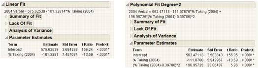
Parameter Estimates Report
The terms in the Parameter Estimates report for a linear fit are the intercept and the single x variable.
For a polynomial fit of order k, there is an estimate for the model intercept and a parameter estimate for each of the k powers of the X variable.
Figure 5.13 Examples of Parameter Estimates Reports for Linear and Polynomial Fits
|
Term
|
Lists the name of each parameter in the requested model. The intercept is a constant term in all models.
|
|
Estimate
|
Lists the parameter estimates of the linear model. The prediction formula is the linear combination of these estimates with the values of their corresponding variables.
|
|
Std Error
|
Lists the estimates of the standard errors of the parameter estimates. They are used in constructing tests and confidence intervals.
|
|
t Ratio
|
Lists the test statistics for the hypothesis that each parameter is zero. It is the ratio of the parameter estimate to its standard error. If the hypothesis is true, then this statistic has a Student’s t-distribution.
|
|
Prob>|t|
|
Lists the observed significance probability calculated from each t-ratio. It is the probability of getting, by chance alone, a t-ratio greater (in absolute value) than the computed value, given a true null hypothesis. Often, a value below 0.05 (or sometimes 0.01) is interpreted as evidence that the parameter is significantly different from zero.
|
To reveal additional statistics, right-click in the report and select the Columns menu. Statistics not shown by default are as follows:
Lower 95%
The lower endpoint of the 95% confidence interval for the parameter estimate.
Upper 95%
The upper endpoint of the 95% confidence interval for the parameter estimate.
Std Beta
The standardized parameter estimate. It is useful for comparing the effect of X variables that are measured on different scales. See “Statistical Details for the Parameter Estimates Report”.
VIF
The variance inflation factor.
Design Std Error
The design standard error for the parameter estimate. See “Statistical Details for the Parameter Estimates Report”.
Fit Special
Using the Fit Special command, you can transform Y and X. Transformations include the following: log, square root, square, reciprocal, and exponential. You can also constrain the slope and intercept, fit a polynomial of specific degree, and center the polynomial.
|
Y Transformation
|
Use these options to transform the Y variable.
|
|
X Transformation
|
Use these options to transform the X variable.
|
|
Degree
|
Use this option to fit a polynomial of the specified degree.
|
|
Centered Polynomial
|
To turn off polynomial centering, deselect the Centered Polynomial check box. See Figure 5.20. Note that for transformations of the X variable, polynomial centering is not performed. Centering polynomials stabilizes the regression coefficients and reduces multicollinearity.
|
|
Constrain Intercept to
|
Select this check box to constrain the model intercept to be the specified value.
|
|
Constrain Slope to
|
Select this check box to constrain the model slope to be the specified value.
|
Fit Special Reports and Menus
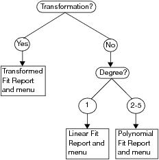
Depending on your selections in the Fit Special window, you see different reports and menus. The flowchart in Figure 5.14 shows you what reports and menus you see depending on your choices.
Figure 5.14 Example of Fit Special Flowchart
Transformed Fit Report
The Transformed Fit report contains the reports described in “Linear Fit and Polynomial Fit Reports”.
However, if you transformed Y, the Fit Measured on Original Scale report appears. This shows the measures of fit based on the original Y variables, and the fitted model transformed back to the original scale.
Fit Spline
Using the Fit Spline command, you can fit a smoothing spline that varies in smoothness (or flexibility) according to the lambda (λ) value. The lambda value is a tuning parameter in the spline formula. As the value of λ decreases, the error term of the spline model has more weight and the fit becomes more flexible and curved. As the value of λ increases, the fit becomes stiff (less curved), approaching a straight line.
Note the following information:
• The smoothing spline can help you see the expected value of the distribution of Y across X.
• The points closest to each piece of the fitted curve have the most influence on it. The influence increases as you lower the value of λ, producing a highly flexible curve.
• If you want to use a lambda value that is not listed on the menu, select Fit Spline > Other. If the scaling of the X variable changes, the fitted model also changes. To prevent this from happening, select the Standardize X option. This option guarantees that the fitted model remains the same for either the original x variable or the scaled X variable.
• You might find it helpful to try several λ values. You can use the Lambda slider beneath the Smoothing Spline report to experiment with different λ values. However, λ is not invariant to the scaling of the data. For example, the λ value for an X measured in inches, is not the same as the λ value for an X measured in centimeters.
Smoothing Spline Fit Report
The Smoothing Spline Fit report contains the R-Square for the spline fit and the Sum of Squares Error. You can use these values to compare the spline fit to other fits, or to compare different spline fits to each other.
|
R-Square
|
Measures the proportion of variation accounted for by the smoothing spline model. For more information, see “Statistical Details for the Smoothing Fit Reports”.
|
|
Sum of Squares Error
|
Sum of squared distances from each point to the fitted spline. It is the unexplained error (residual) after fitting the spline model.
|
|
Change Lambda
|
Enables you to change the λ value, either by entering a number, or by moving the slider.
|
Kernel Smoother
The Kernel Smoother command produces a curve formed by repeatedly finding a locally weighted fit of a simple curve (a line or a quadratic) at sampled points in the domain. The many local fits (128 in total) are combined to produce the smooth curve over the entire domain. This method is also called Loess or Lowess, which was originally an acronym for Locally Weighted Scatterplot Smoother. See Cleveland (1979).
Use this method to quickly see the relationship between variables and to help you determine the type of analysis or fit to perform.
Local Smoother Report
The Local Smoother report contains the R-Square for the kernel smoother fit and the Sum of Squares Error. You can use these values to compare the kernel smoother fit to other fits, or to compare different kernel smoother fits to each other.
|
R-Square
|
Measures the proportion of variation accounted for by the kernel smoother model. For more information, see “Statistical Details for the Smoothing Fit Reports”.
|
|
Sum of Squares Error
|
Sum of squared distances from each point to the fitted kernel smoother. It is the unexplained error (residual) after fitting the kernel smoother model.
|
|
Local Fit (lambda)
|
Select the polynomial degree for each local fit. Quadratic polynomials can track local bumpiness more smoothly. Lambda is the degree of certain polynomials that are fitted by the method. Lambda can be 1 or 2.
|
|
Weight Function
|
Specify how to weight the data in the neighborhood of each local fit. Loess uses tri-cube. The weight function determines the influence that each xi and yi has on the fitting of the line. The influence decreases as xi increases in distance from x and finally becomes zero.
|
|
Smoothness (alpha)
|
Controls how many points are part of each local fit. Use the slider or type in a value directly. Alpha is a smoothing parameter. It can be any positive number, but typical values are 1/4 to 1. As alpha increases, the curve becomes smoother.
|
|
Robustness
|
Reweights the points to deemphasize points that are farther from the fitted curve. Specify the number of times to repeat the process (number of passes). The goal is to converge the curve and automatically filter out outliers by giving them small weights.
|
Fit Each Value
The Fit Each Value command fits a value to each unique X value. The fitted values are the means of the response for each unique X value.
Fit Each Value Report
The Fit Each Value report shows summary statistics about the model fit.
|
Number of Observations
|
Gives the total number of observations.
|
|
Number of Unique Values
|
Gives the number of unique X values.
|
|
Degrees of Freedom
|
Gives the pure error degrees of freedom.
|
|
Sum of Squares
|
Gives the pure error sum of squares.
|
|
Mean Square
|
Gives the pure error mean square.
|
Fit Orthogonal
The Fit Orthogonal command fits lines that adjust for variability in X as well as Y.
Fit Orthogonal Options
The following table describes the available options to specify a variance ratio.
|
Univariate Variances, Prin Comp
|
Uses the univariate variance estimates computed from the samples of X and Y. This turns out to be the standardized first principal component. This option is not a good choice in a measurement systems application since the error variances are not likely to be proportional to the population variances.
|
|
Equal Variances
|
Uses 1 as the variance ratio, which assumes that the error variances are the same. Using equal variances is equivalent to the non-standardized first principal component line. Suppose that the scatterplot is scaled the same in the X and Y directions. When you show a normal density ellipse, you see that this line is the longest axis of the ellipse.
|
|
Fit X to Y
|
Uses a variance ratio of zero, which indicates that Y effectively has no variance.
|
|
Specified Variance Ratio
|
Lets you enter any ratio that you want, giving you the ability to make use of known information about the measurement error in X and response error in Y.
|
Orthogonal Regression Report
The Orthogonal Regression report shows summary statistics about the orthogonal regression model.
The following table describes the Orthogonal Regression report.
|
Variable
|
Gives the names of the variables used to fit the line.
|
|
Mean
|
Gives the mean of each variable.
|
|
Std Dev
|
Gives the standard deviation of each variable.
|
|
Variance Ratio
|
Gives the variance ratio used to fit the line.
|
|
Correlation
|
Gives the correlation between the two variables.
|
|
Intercept
|
Gives the intercept of the fitted line.
|
|
Slope
|
Gives the slope of the fitted line.
|
|
LowerCL
|
Gives the lower confidence limit for the slope.
|
|
UpperCL
|
Gives the upper confidence limit for the slope.
|
|
Alpha
|
Enter the alpha level used in computing the confidence interval.
|
Density Ellipse
Using the Density Ellipse option, you can draw an ellipse (or ellipses) that contains the specified mass of points. The number of points is determined by the probability that you select from the Density Ellipse menu).
Figure 5.15 Example of Density Ellipses
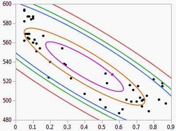
The density ellipsoid is computed from the bivariate normal distribution fit to the X and Y variables. The bivariate normal density is a function of the means and standard deviations of the X and Y variables and the correlation between them. The Other selection lets you specify any probability greater than zero and less than or equal to one.
These ellipses are both density contours and confidence curves. As confidence curves, they show where a given percentage of the data is expected to lie, assuming the bivariate normal distribution.
The density ellipsoid is a good graphical indicator of the correlation between two variables. The ellipsoid collapses diagonally as the correlation between the two variables approaches either 1 or –1. The ellipsoid is more circular (less diagonally oriented) if the two variables are less correlated.
Correlation Report
The Correlation report that accompanies each Density Ellipse fit shows the correlation coefficient for the X and Y variables.
Note: To see a matrix of ellipses and correlations for many pairs of variables, use the Multivariate command in the Analyze > Multivariate Methods menu.
|
Variable
|
Gives the names of the variables used in creating the ellipse
|
|
Mean
|
Gives the average of both the X and Y variable.
|
|
Std Dev
|
Gives the standard deviation of both the X and Y variable.
A discussion of the mean and standard deviation are in the section “The Summary Statistics Report” in the “Distributions” chapter.
|
|
Correlation
|
The Pearson correlation coefficient. If there is an exact linear relationship between two variables, the correlation is 1 or –1 depending on whether the variables are positively or negatively related. If there is no relationship, the correlation tends toward zero.
For more information, see “Statistical Details for the Correlation Report”.
|
|
Signif. Prob
|
Probability of obtaining, by chance alone, a correlation with greater absolute value than the computed value if no linear relationship exists between the X and Y variables.
|
|
Number
|
Gives the number of observations used in the calculations.
|
Nonpar Density
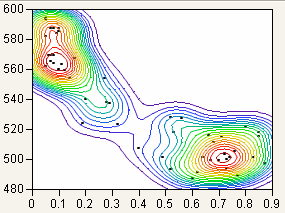
When a plot shows thousands of points, the mass of points can be too dark to show patterns in density. Using the Nonpar Density (nonparametric density) option makes it easier to see the patterns.
Bivariate density estimation models a smooth surface that describes how dense the data points are at each point in that surface. The plot adds a set of contour lines showing the density (Figure 5.16). The contour lines are quantile contours in 5% intervals. This means that about 5% of the points are below the lowest contour, 10% are below the next contour, and so on. The highest contour has about 95% of the points below it.
Figure 5.16 Example of Nonpar Density
Nonparametric Bivariate Density Report
The nonparametric bivariate density report shows the kernel standard deviations used in creating the nonparametric density.
Fit Robust
Note: For more details about robust fitting, see Huber, 1973.
The Fit Robust option attempts to reduce the influence of outliers in your data set. In this instance, outliers are an observation that does not come from the “true” underlying distribution of the data. For example, if weight measurements were being taken in pounds for a sample of individuals, but one of the individuals accidentally recorded their weight in kilograms instead of pounds, this would be a deviation from the true distribution of the data. Outliers such as this could lead you into making incorrect decisions because of their influence on the data. The Fit Robust option reduces the influence of these types of outliers.
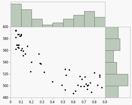
Histogram Borders
The Histogram Borders option appends histograms to the x- and y-axes of the scatterplot. You can use the histograms to visualize the marginal distributions of the X and Y variables.
Figure 5.17 Example of Histogram Borders
Group By
Using the Group By option, you can select a classification (grouping) variable. When a grouping variable is in effect, the Bivariate platform computes a separate analysis for each level of the grouping variable. Regression curves or ellipses then appear on the scatterplot. The fit for each level of the grouping variable is identified beneath the scatterplot, with individual popup menus to save or remove fitting information.
The Group By option is checked in the Fitting menu when a grouping variable is in effect. You can change the grouping variable by first selecting the Group By option to remove (uncheck) the existing variable. Then, select the Group By option again and respond to its window as before.
You might use the Group By option in these different ways:
• An overlay of linear regression lines lets you compare slopes visually.
• An overlay of density ellipses can show clusters of points by levels of a grouping variable.
Fitting Menus
In addition to a report, each fitting command adds a fitting menu to the report window. The following table shows the fitting menus that correspond to each fitting command.
|
Fitting Command
|
Fitting Menu
|
|
Fit Mean
|
Fit Mean
|
|
Fit Line
|
Linear Fit
|
|
Fit Polynomial
|
Polynomial Fit Degree=X*
|
|
Fit Special
|
Linear Fit
Polynomial Fit Degree=X*
Transformed Fit X*
Constrained Fits
|
|
Fit Spline
|
Smoothing Spline Fit, lambda=X*
|
|
Kernel Smoother
|
Local Smoother
|
|
Fit Each Value
|
Fit Each Value
|
|
Fit Orthogonal
|
Orthogonal Fit Ratio=X*
|
|
Density Ellipse
|
Bivariate Normal Ellipse P=X*
|
|
Nonpar Density
|
Quantile Density Colors
|
|
Fit Robust
|
Robust Fit
|
*X=variable character or number
Fitting Menu Options
The following table describes the options in the Fitting menus.
|
Confid Curves Fit
|
Displays or hides the confidence limits for the expected value (mean). This option is not available for the Fit Spline, Density Ellipse, Fit Each Value, and Fit Orthogonal fits and is dimmed on those menus.
|
|
Confid Curves Indiv
|
Displays or hides the confidence limits for an individual predicted value. The confidence limits reflect variation in the error and variation in the parameter estimates. This option is not available for the Fit Mean, Fit Spline, Density Ellipse, Fit Each Value, and Fit Orthogonal fits and is dimmed on those menus.
|
|
Line Color
|
Lets you select from a palette of colors for assigning a color to each fit.
|
|
Line of Fit
|
Displays or hides the line of fit.
|
|
Line Style
|
Lets you select from the palette of line styles for each fit.
|
|
Line Width
|
Gives three line widths for the line of fit. The default line width is the thinnest line.
|
|
Report
|
Turns the fit’s text report on and off.
|
|
Save Predicteds
|
Creates a new column in the current data table called Predicted colname where colname is the name of the Y variable. This column includes the prediction formula and the computed sample predicted values. The prediction formula computes values automatically for rows that you add to the table. This option is not available for the Fit Each Value and Density Ellipse fits and is dimmed on those menus.
Note: You can use the Save Predicteds and Save Residuals commands for each fit. If you use these commands multiple times or with a grouping variable, it is best to rename the resulting columns in the data table to reflect each fit.
|
|
Save Residuals
|
Creates a new column in the current data table called Residuals colname where colname is the name of the Y variable. Each value is the difference between the actual (observed) value and its predicted value. Unlike the Save Predicteds command, this command does not create a formula in the new column. This option is not available for the Fit Each Value and Density Ellipse fits and is dimmed on those menus.
Note: You can use the Save Predicteds and Save Residuals commands for each fit. If you use these commands multiple times or with a grouping variable, it is best to rename the resulting columns in the data table to reflect each fit.
|
|
Remove Fit
|
Removes the fit from the graph and removes its text report.
|
|
Linear Fits, Polynomial Fits, and Fit Special, and Fit Robust Only:
|
|
|
Mean Confidence Limit Formula
|
Creates a new column in the data table containing a formula for the mean confidence intervals.
|
|
Indiv Confidence Limit Formula
|
Creates a new column in the data table containing a formula for the individual confidence intervals.
|
|
Confid Shaded Fit
|
Draws the same curves as the Confid Curves Fit command and shades the area between the curves.
|
|
Confid Shaded Indiv
|
Draws the same curves as the Confid Curves Indiv command and shades the area between the curves.
|
|
Plot Residuals
|
Produces four diagnostic plots: residual by predicted, actual by predicted, residual by row, and a normal quantile plot of the residuals. See “Diagnostics Plots”.
|
|
Set Alpha Level
|
Prompts you to enter the alpha level to compute and display confidence levels for line fits, polynomial fits, and special fits.
|
|
Smoothing Spline Fit and Local Smoother Only:
|
|
|
Save Coefficients
|
Saves the spline coefficients as a new data table, with columns called X, A, B, C, and D. The X column gives the knot points. A, B, C, and D are the intercept, linear, quadratic, and cubic coefficients of the third-degree polynomial. These coefficients span from the corresponding value in the X column to the next highest value.
|
|
Bivariate Normal Ellipse Only:
|
|
|
Shaded Contour
|
Shades the area inside the density ellipse.
|
|
Select Points Inside
|
Selects the points inside the ellipse.
|
|
Select Points Outside
|
Selects the points outside the ellipse.
|
|
Quantile Density Contours Only:
|
|
|
Kernel Control
|
Displays a slider for each variable, where you can change the kernel standard deviation that defines the range of X and Y values for determining the density of contour lines.
|
|
5% Contours
|
Shows or hides the 5% contour lines.
|
|
Contour Lines
|
Shows or hides the contour lines.
|
|
Contour Fill
|
Fills the areas between the contour lines.
|
|
Select Points by Density
|
Selects points that fall in a user-specified quantile range.
|
|
Color by Density Quantile
|
Colors the points according to density.
|
|
Save Density Quantile
|
Creates a new column containing the density quantile each point is in.
|
|
Mesh Plot
|
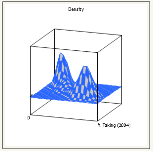
Is a three-dimensional plot of the density over a grid of the two analysis variables. See Figure 5.18.
|
|
Model Clustering
|
Creates a new column in the current data table and fills it with cluster values.
Note: If you save the modal clustering values first and then save the density grid, the grid table also contains the cluster values. The cluster values are useful for coloring and marking points in plots.
|
|
Save Density Grid
|
Saves the density estimates and the quantiles associated with them in a new data table. The grid data can be used to visualize the density in other ways, such as with the Scatterplot 3D or the Contour Plot platforms.
|
Figure 5.18 Example of a Mesh Plot
Diagnostics Plots
The Plot Residuals option creates residual plots and other plots to diagnose the model fit. The following plots are available:
Residual by Predicted Plot
is a plot of the residuals vs. the predicted values. A histogram of the residuals is also created.
Actual by Predicted Plot
is a plot of the actual values vs. the predicted values.
Residual by Row Plot
is a plot of the residual values vs. the row number.
Residual by X Plot
is a plot of the residual values vs. the X variable.
Residual Normal Quantile Plot
is a Normal quantile plot of the residuals.
Additional Examples of the Bivariate Platform
This section contains additional examples using the fitting commands in the Bivariate platform.
Example of the Fit Special Command
To transform Y as log and X as square root, proceed as follows:
1. Open the SAT.jmp sample data table.
2. Select Analyze > Fit Y by X.
3. Select 2004 Verbal and click Y, Response.
4. Select % Taking (2004) and click X, Factor.
5. Click OK.
Figure 5.19 Example of SAT Scores by Percent Taking
6. From the red triangle menu for Bivariate Fit, select Fit Special. The Specify Transformation or Constraint window appears. For a description of this window, see Table 5.8.
Figure 5.20 The Specify Transformation or Constraint Window
7. Within Y Transformation, select Natural Logarithm: log(y).
8. Within X Transformation, select Square Root: sqrt(x).
9. Click OK.
Figure 5.21 Example of Fit Special Report
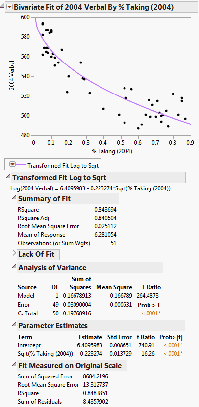
Figure 5.21 shows the fitted line plotted on the original scale. The model appears to fit the data well, as the plotted line goes through the cloud of points.
Example Using the Fit Orthogonal Command
This example involves two parts. First, standardize the variables using the Distribution platform. Then, use the standardized variables to fit the orthogonal model.
Standardize the Variables
1. Open the Big Class.jmp sample data table.
2. Select Analyze > Distribution.
3. Select height and weight and click Y, Columns.
4. Click OK.
5. Hold down the CTRL key. On the red triangle menu next to height, select Save > Standardized.
Holding down the CTRL key broadcasts the operation to all variables in the report window. Notice that in the Big Class.jmp sample data table, two new columns have been added.
6. Close the Distribution report window.
Use the Standardized Variables to Fit the Orthogonal Model
1. From the Big Class.jmp sample data table, select Analyze > Fit Y by X.
2. Select Std weight and click Y, Response.
3. Select Std height and click X, Factor.
4. Click OK.
5. From the red triangle menu, select Fit Line.
6. From the red triangle menu, select Fit Orthogonal. Then select each of the following:
‒ Equal Variances
‒ Fit X to Y
‒ Specified Variance Ratio and type 0.2.
‒ Specified Variance Ratio and type 5.
Figure 5.22 Example of Orthogonal Fitting Options
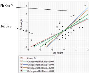
The scatterplot in Figure 5.22 shows the standardized height and weight values with various line fits that illustrate the behavior of the orthogonal variance ratio selections. The standard linear regression (Fit Line) occurs when the variance of the X variable is considered to be very small. Fit X to Y is the opposite extreme, when the variation of the Y variable is ignored. All other lines fall between these two extremes and shift as the variance ratio changes. As the variance ratio increases, the variation in the Y response dominates and the slope of the fitted line shifts closer to the Y by X fit. Likewise, when you decrease the ratio, the slope of the line shifts closer to the X by Y fit.
Example Using the Fit Robust Command
The data in the Weight Measurements.jmp sample data table shows the height and weight measurements taken by 40 students.
1. Open the Weight Measurements.jmp sample data table.
2. Select Analyze > Fit Y by X.
3. Select weight and click Y, Response.
4. Select height and click X, Factor.
5. Click OK.
6. From the red triangle menu, select Fit Line.
7. From the red triangle menu, select Fit Robust.
Figure 5.23 Example of Robust Fit
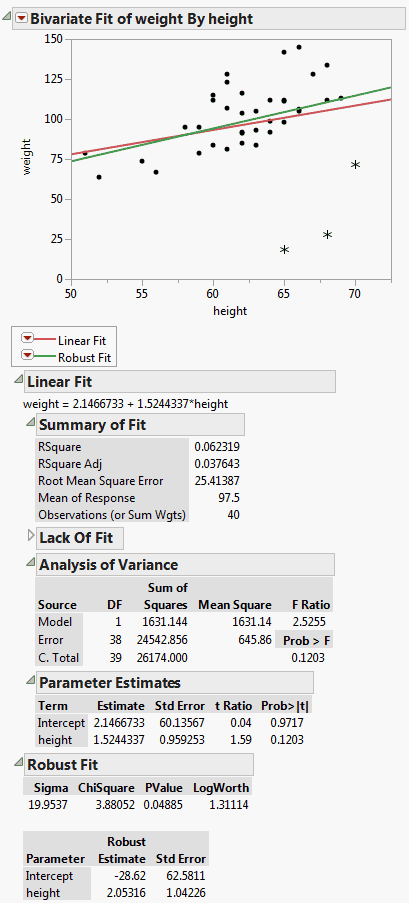
If you look at the standard Analysis of Variance report, you might wrongly conclude that height and weight do not have a linear relationship, since the p-value is 0.1203. However, when you look at the Robust Fit report, you would probably conclude that they do have a linear relationship, because the p-value there is 0.0489. It appears that some of the measurements are unusually low, perhaps due to incorrect user input. These measurements were unduly influencing the analysis.
Example of Group By Using Density Ellipses
This example uses the Hot Dogs.jmp sample data table. The Type column identifies three different types of hot dogs: beef, meat, or poultry. You want to group the three types of hot dogs according to their cost variables.
1. Open the Hot Dogs.jmp sample data table.
2. Select Analyze > Fit Y by X.
3. Select $/oz and click Y, Response.
4. Select $/lb Protein and click X, Factor.
5. Click OK.
6. From the red triangle menu, select Group By.
7. From the list, select Type.
8. Click OK. If you look at the Group By option again, you see it has a check mark next to it.
9. From the red triangle menu, select Density Ellipse > 0.90.
To color the points according to Type, proceed as follows:
10. Right-click on the scatterplot and select Row Legend.
11. Select Type in the column list and click OK.
Figure 5.24 Example of Group By
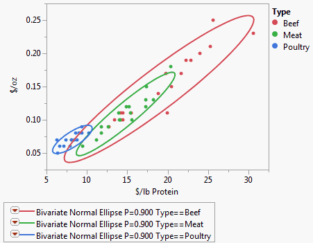
The ellipses in Figure 5.24 show clearly how the different types of hot dogs cluster with respect to the cost variables.
Example of Group By Using Regression Lines
Another use for grouped regression is overlaying lines to compare slopes of different groups.
1. Open the Big Class.jmp sample data table.
2. Select Analyze > Fit Y by X.
3. Select weight and click Y, Response.
4. Select height and click X, Factor.
5. Click OK.
To create the example on the left in Figure 5.25:
6. Select Fit Line from the red triangle menu.
To create the example on the right in Figure 5.25:
7. From the Linear Fit menu, select Remove Fit.
8. From the red triangle menu, select Group By.
9. From the list, select sex.
10. Click OK.
11. Select Fit Line from the red triangle menu.
Figure 5.25 Example of Regression Analysis for Whole Sample and Grouped Sample
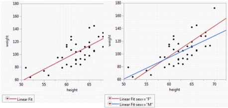
The scatterplot to the left in Figure 5.25 has a single regression line that relates weight to height. The scatterplot to the right shows separate regression lines for males and females.
Statistical Details for the Bivariate Platform
This section contains statistical details for selected commands and reports.
Statistical Details for Fit Line
The Fit Line command finds the parameters  and
and  for the straight line that fits the points to minimize the residual sum of squares. The model for the ith row is written
 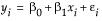 .
.
A polynomial of degree 2 is a parabola; a polynomial of degree 3 is a cubic curve. For degree k, the model for the ith observation is as follows:

Statistical Details for Fit Spline
The cubic spline method uses a set of third-degree polynomials spliced together such that the resulting curve is continuous and smooth at the splices (knot points). The estimation is done by minimizing an objective function that is a combination of the sum of squares error and a penalty for curvature integrated over the curve extent. See the paper by Reinsch (1967) or the text by Eubank (1988) for a description of this method.
Statistical Details for Fit Orthogonal
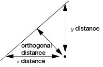
Standard least square fitting assumes that the X variable is fixed and the Y variable is a function of X plus error. If there is random variation in the measurement of X, you should fit a line that minimizes the sum of the squared perpendicular differences. See Figure 5.26. However, the perpendicular distance depends on how X and Y are scaled, and the scaling for the perpendicular is reserved as a statistical issue, not a graphical one.
Figure 5.26 Line Perpendicular to the Line of Fit
The fit requires that you specify the ratio of the variance of the error in Y to the error in X. This is the variance of the error, not the variance of the sample points, so you must choose carefully. The ratio  is infinite in standard least squares because
  is zero. If you do an orthogonal fit with a large error ratio, the fitted line approaches the standard least squares line of fit. If you specify a ratio of zero, the fit is equivalent to the regression of X on Y, instead of Y on X.
The most common use of this technique is in comparing two measurement systems that both have errors in measuring the same value. Thus, the Y response error and the X measurement error are both the same type of measurement error. Where do you get the measurement error variances? You cannot get them from bivariate data because you cannot tell which measurement system produces what proportion of the error. So, you either must blindly assume some ratio like 1, or you must rely on separate repeated measurements of the same unit by the two measurement systems.
An advantage to this approach is that the computations give you predicted values for both Y and X; the predicted values are the point on the line that is closest to the data point, where closeness is relative to the variance ratio.
Confidence limits are calculated as described in Tan and Iglewicz (1999).
Statistical Details for the Summary of Fit Report
Rsquare
Using quantities from the corresponding analysis of variance table, the Rsquare for any continuous response fit is calculated as follows:
RSquare Adj
The RSquare Adj is a ratio of mean squares instead of sums of squares and is calculated as follows:
The mean square for Error is in the Analysis of Variance report. See Figure 5.12. You can compute the mean square for C. Total as the Sum of Squares for C. Total divided by its respective degrees of freedom.
Statistical Details for the Lack of Fit Report
Pure Error DF
For the Pure Error DF, consider the multiple instances in the Big Class.jmp sample data table where more than one subject has the same value of height. In general, if there are g groups having multiple rows with identical values for each effect, the pooled DF, denoted DFp, is as follows:
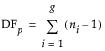
ni is the number of subjects in the ith group.
Pure Error SS
For the Pure Error SS, in general, if there are g groups having multiple rows with the same x value, the pooled SS, denoted SSp, is written as follows:

where SSi is the sum of squares for the ith group corrected for its mean.
Max RSq
Because Pure Error is invariant to the form of the model and is the minimum possible variance, Max RSq is calculated as follows:
Statistical Details for the Parameter Estimates Report
Std Beta
Std Beta is calculated as follows:
where  is the estimated parameter, sx and sy are the standard deviations of the X and Y variables.
Design Std Error
Design Std Error is calculated as the standard error of the parameter estimate divided by the RMSE.
Statistical Details for the Smoothing Fit Reports
R-Square is equal to 1-(SSE/C.Total SS), where C.Total SS is available in the Fit Line ANOVA report.
Statistical Details for the Correlation Report
The Pearson correlation coefficient is denoted r, and is computed as follows:
 where
whereWhere  is either the weight of the ith observation if a weight column is specified, or 1 if no weight column is assigned.
..................Content has been hidden....................
You can't read the all page of ebook, please click here login for view all page.