
Example of the Tabulate Platform
You have data containing height measurements for male and female students. You want to create a table that shows the mean height for males and females and the aggregate mean for both sexes. You want the table to look Figure 11.2.
Figure 11.2 Table Showing Mean Height
1. Open the Big Class.jmp sample data table.
2. Select Analyze > Tabulate.
Since height is the variable you are examining, you want it to appear at the top of the table.
3. Click height and drag it into the Drop zone for columns.
Figure 11.3 Height Variable Added
You want the statistics by sex, and you want sex to appear on the side.
4. Click sex and drag it into the blank cell next to the number 2502.0.
Figure 11.4 Sex Variable Added
Instead of the sum, you want it to show the mean.
5. Click Mean and drag it on top of Sum.
Figure 11.5 Mean Statistic Added
You also want to see the combined mean for males and females.
6. Click All and drag it on top of sex. Or, you can simply select the Add Aggregate Statistics check box.
Figure 11.6 All Statistic Added
7. (Optional) Click Done.
The completed table shows the mean height for females, males, and the combined mean height for both.
Launch the Tabulate Platform
To launch the Tabulate platform, select Analyze > Tabulate.
Figure 11.7 The Tabulate Interactive Table
Note: For details about red triangle options, see “Tabulate Platform Options”.
The Tabulate window contains the following options:
Interactive table/dialog
Switch between the two modes. Use the interactive table mode to drag and drop items, creating a custom table. Use the dialog mode to create a simple table using a fixed format. See “Use the Dialog”.
Statistics options
Lists standard statistics. Drag any statistic from the list to the table to incorporate it. See “Add Statistics”.
Drop zone for columns
Drag and drop columns or statistics here to create columns.
Drop zone for rows
Drag and drop columns or statistics here to create rows.
Resulting cells
Shows the resulting cells based on the columns or statistics that you drag and drop.
Freq
Identifies the data table column whose values assign a frequency to each row. This option is useful when a frequency is assigned to each row in summarized data.
Weight
Identifies the data table column whose variables assign weight (such as importance or influence) to the data.
Page Column
Generates separate tables for each category of a nominal or ordinal column. See “Example Using a Page Column”.
Include missing for grouping columns
Creates a separate group for missing values in grouping columns. When unchecked, missing values are not included in the table. Note that any missing value codes that you have defined as column properties are taken into account.
Order by count of grouping columns
Changes the order of the table to be in ascending order of the values of the grouping columns.
Add Aggregate Statistics
Adds aggregate statistics for all rows and columns.
Default Statistics
Enables you to change the default statistics that appear when you drag and drop analysis or non-analysis (for example, grouping) columns.
Change Format
Enables you to change the numeric format for displaying specific statistics. See “Delete Items”.
Change Plot Scale
(Only appears if Show Chart is selected from the red triangle menu.) Enables you to specify a uniform custom scale.
Uniform plot scale
(Only appears if Show Chart is selected from the red triangle menu.) Deselect this box for each column of bars to use the scale determined separately from the data in each displayed column.
Use the Dialog
If you prefer not to drag and drop and build the table interactively, you can create a simple table using the Dialog interface. After selecting Analyze > Tabulate, select Dialog from the menu, as shown in Figure 11.8. You can make changes to the table by selecting Show Control Panel from the red triangle menu, and then drag and drop new items into the table.
Figure 11.8 Using the Dialog
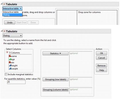
The dialog contains the following options:
Include marginal statistics
Aggregates summary information for categories of a grouping column.
For quantile statistics, enter value (%)
Type the value at which the specific percentage of the argument is less than or equal to. For example, 75% of the data is less than the 75th quantile. This applies to all grouping columns.
Statistics
Once you’ve selected a column, select a standard statistic to apply to that column. See “Add Statistics”
Grouping (row labels)
Select the column to use as the row label.
Grouping (column labels)
Select the column to use as the column label.
Add Statistics
Tip: You can select both a column and a statistic at the same time and drag them into the table.
Tabulate supports a list of standard statistics. The list is displayed in the control panel. You can drag any keyword from that list to the table, just like you do with the columns. Note the following:
• The statistics associated with each cell are calculated on values of the analysis columns from all observations in that category, as defined by the grouping columns.
• All of the requested statistics have to reside in the same dimension, either in the row table or in the column table.
• If you drag a continuous column into a data area, it is treated as an analysis column.
Tabulate uses the following keywords:
N
Provides the number of nonmissing values in the column. This is the default statistic when there is no analysis column.
Mean
Provides the arithmetic mean of a column’s values. It is the sum of nonmissing values (and if defined, multiplied by the weight variable) divided by the Sum Wgt.
Std Dev
Provides the sample standard deviation, computed for the nonmissing values. It is the square root of the sample variance.
Min
Provides the smallest nonmissing value in a column.
Max
Provides the largest nonmissing value in a column.
Range
Provides the difference between Max and Min.
% of Total
Computes the percentage of total of the whole population. The denominator used in the computation is the total of all the included observations, and the numerator is the total for the category. If there is no analysis column, the % of Total is the percentage of total of counts. If there is an analysis column, the % of Total is the percentage of the total of the sum of the analysis column. Thus, the denominator is the sum of the analysis column over all the included observations, and the numerator is the sum of the analysis column for that category. You can request different percentages by dragging the keyword into the table.
‒ Dropping one or more grouping columns from the table to the % of Total heading changes the denominator definition. For this, Tabulate uses the sum of these grouping columns for the denominator.
‒ To get the percentage of the column total, drag all the grouping columns on the row table and drop them onto the % of Total heading (same as Column %). Similarly, to get the percentage of the row total, drag all grouping columns on the column table and drop them onto the % of Total heading (same as Row %).
N Missing
Provides the number of missing values.
N Categories
Provides the number of distinct categories.
Sum
Provides the sum of all values in the column. This is the default statistic for analysis columns when there are no other statistics for the table.
Sum Wgt
Provides the sum of all weight values in a column. Or, if no column is assigned the weight role, Sum Wgt is the total number of nonmissing values.
Variance
Provides the sample variance, computed for the nonmissing values. It is the sum of squared deviations from the mean, divided by the number of nonmissing values minus one.
Std Err
Provides the standard error of the mean. It is the standard deviation divided by the square root of N. If a column is assigned the role of weight, then the denominator is the square root of the sum of the weights.
CV
(Coefficient of Variation) Provides the measure of dispersion, which is the standard deviation divided by the mean multiplied by one hundred.
Median
Provides the 50th percentile, which is the value where half the data are below and half are above or equal to the 50th quantile (median).
Interquartile Range
Provides the difference between the 3rd quartile and 1st quartile.
Quantiles
Provides the value at which the specific percentage of the argument is less than or equal to. For example, 75% of the data is less than the 75th quantile. You can request different quantiles by clicking and dragging the Quantiles keyword into the table, and then entering the quantile into the box that appears.
Column %
Provides the percent of each cell count to its column total if there is no analysis column. If there is an analysis column, the Column % is the percent of the column total of the sum of the analysis column. For tables with statistics on the top, you can add Column % to tables with multiple row tables (stacked vertically).
Row %
Provides the percent of each cell count to its row total if there is no analysis column. If there is an analysis column, the Row % is the percent of the row total of the sum of the analysis column. For tables with statistics on the side, you can add Row % to tables with multiple row tables (side by side tables).
All
Aggregates summary information for categories of a grouping column.
Change Numeric Formats
The formats of each cell depend on the analysis column and the statistics. For counts, the default format has no decimal digits. For each cell defined by some statistics, JMP tries to determine a reasonable format using the format of the analysis column and the statistics requested. To override the default format:
1. Click the Change Format button at the bottom of the Tabulate window.
2. In the panel that appears, enter the field width, a comma, and then the number of decimal places that you want displayed in the table. See Figure 11.9.
3. (Optional) If you would like JMP to determine the best format for you to use, type the word Best in the text box.
JMP now considers the precision of each cell value and selects the best way to show it.
4. Click OK to implement the changes and close the Format section, or click Set Format to see the changes implemented without closing the Format section.
Figure 11.9 Changing Numeric Formats
The Tabulate Output
The Tabulate output consists of one or more column tables concatenated side by side, and one or more row tables concatenated top to bottom. The output might have only a column table or a row table.
Figure 11.10 Tabulate Output
Creating a table interactively is an iterative process:
• Click the items (columns or statistics) from the appropriate list, and drag them into the drop zone (for rows or columns). See “Edit Tables”, and “Column and Row Tables”.
• Add to the table by repeating the drag and drop process. The table updates to reflect the latest addition. If there are already column headings or row labels, you can decide where the addition goes relative to the existing items.
Note the following about clicking and dragging:
• JMP uses the modeling type to determine a column’s role. Continuous columns are assumed to be analysis columns. See “Analysis Columns”. Ordinal or nominal columns are assumed to be grouping columns. See “Grouping Columns”.
• When you drag and drop multiple columns into the initial table:
‒ If the columns share a set of common values, they are combined into a single table. A crosstabulation of the column names and the categories gathered from these columns is generated. Each cell is defined by one of the columns and one of the categories.
‒ If the columns do not share common values, they are put into separate tables.
‒ You can always change the default action by right-clicking on a column and selecting Combine Tables or Separate Tables. For more details, see “Right-Click Menu for Columns”.
• To nest columns, create a table with the first column, and then drag the additional columns into the first column.
• In a properly created table, all grouping columns are together, all analysis columns are together, and all statistics are together. Therefore, JMP does not intersperse a statistics keyword within a list of analysis columns. JMP also does not insert an analysis column within a list of grouping columns.
• You can drag columns from the Table panel in the data table onto a Tabulate table instead of using the Tabulate Control Panel.
Analysis Columns
Analysis columns are any numeric columns for which you want to compute statistics. They are continuous columns. Tabulate computes statistics on the analysis columns for each category formed from the grouping columns.
Note that all the analysis columns have to reside in the same dimension, either in the row table or in the column table.
Grouping Columns
Grouping columns are columns that you want to use to classify your data into categories of information. They can have character, integer, or even decimal values, but the number of unique values should be limited. Grouping columns are either nominal or ordinal.
Note the following:
• If grouping columns are nested, Tabulate constructs distinct categories from the hierarchical nesting of the values of the columns. For example, from the grouping columns Sex with values F and M, and the grouping column Marital Status with values Married and Single, Tabulate constructs four distinct categories: F and Married, F and Single, M and Married, M and Single.
• You can specify grouping columns for column tables as well as row tables. Together they generate the categories that define each table cell.
• Tabulate does not include observations with a missing value for one or more grouping columns by default. You can include them by checking the Include missing for grouping columns option.
• To specify codes or values that should be treated as missing, use the Missing Value Codes column property. You can include these by checking the Include missing for grouping columns option. For more details about Missing Value Codes, see the Using JMP book.
Column and Row Tables
In Tabulate, a table is defined by its column headings and row labels. These sub-tables are referred to as row tables and column tables. See Figure 11.11.
Example of Row and Column Tables
1. Open the Car Poll.jmp sample data table.
2. Select Analyze > Tabulate.
3. Drag size into the Drop zone for rows.
4. Drag country to the left of the size heading.
5. Drag Mean over the N heading.
6. Drag Std Dev below the Mean heading.
7. Drag age above the Mean heading.
8. Drag type to the far right of the table.
9. Drag sex under the table.
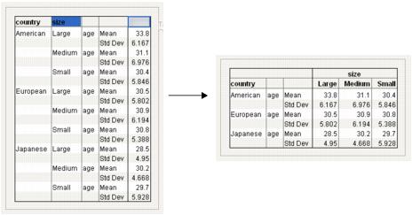
Figure 11.11 Row and Column Tables
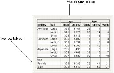
For multiple column tables, the labels on the side are shared across the column tables. In this instance, country and sex are shared across the tables. Similarly, for multiple row tables, the headings on the top are shared among the row tables. In this instance, both age and type are shared among the tables.
Edit Tables
There are several ways to edit the items that you add to a table.
Delete Items
After you add items to the table, you can remove them in any one of the following ways:
• Drag the item away from the table.
• To remove the last item, click Undo.
• Right-click on an item and select Delete.
Remove Column Labels
Grouping columns display the column name on top of the categories associated with that column. For some columns, the column name might seem redundant. Remove the column name from the column table by right-clicking on the column name and selecting Remove Column Label. To re-insert the column label, right-click on one of its associated categories and select Restore Column Label.
Edit Statistical Key Words and Labels
You can edit a statistical key word or a statistical label. For example, instead of Mean, you might want to use the word Average. Right-click on the word that you want to edit and select Change Item Label. In the box that appears, type the new label. Alternatively, you can type directly into the edit box.
If you change one statistics keyword to another statistics keyword, JMP assumes that you actually want to change the statistics, not just the label. It would be as if you have deleted the statistics from the table and added the latter.
Tabulate Platform Options
The following options are available from the red triangle menu next to Tabulate:
Show Table
Displays the summarized data in tabular form.
Show Chart
Displays the summarized data in bar charts that mirrors the table of summary statistics. The simple bar chart enables visual comparison of the relative magnitude of the summary statistics. By default, all columns of bars share the same scale. You can have each column of bars use the scale determined separately from the data in each displayed column, by clearing the Uniform plot scale check box. You can specify a uniform custom scale using the Change Plot Scale button. The charts are either 0-based or centered on 0. If the data are all nonnegative, or all non-positive, the charts baseline is at 0. Otherwise, the charts are centered on 0.
Show Control Panel
Displays the control panel for further interaction.
Show Shading
Displays gray shading boxes in the table when there are multiple rows.
Show Tooltip
Displays tips that appear when you move the mouse over areas of the table.
Show Test Build Panel
Displays the control area that lets you create a test build using a random sample from the original table. This is particularly useful when you have large amounts of data. See “Show Test Build Panel”.
Make Into Data Table
Makes a data table from the report. There is one data table for each row table, because labels of different row tables might not be mapped to the same structure.
Script
Displays options for saving scripts, redoing analyses, and viewing the data table. For details, see the Using JMP book.
Note: For a description of the options in the Select Columns red triangle menu, see the Using JMP book.
Show Test Build Panel
If you have a very large data table, you might want to use a small subset of the data table to try out different table layouts to find one that best shows the summary information. In this case, JMP generates a random subset of the size as specified and uses that subset when it builds the table. To use the test build feature:
1. From the red triangle menu next to Tabulate, select Show Test Build Panel.
2. Enter the size of the sample that you want in the box under Sample Size (>1) or Sampling Rate (<1), as shown in Figure 11.12. The size of the sample can be either the proportion of the active table that you enter or the number of rows from the active table.
Figure 11.12 The Test Build Panel
3. Click Resample.
4. To see the sampled data in a JMP data table, click the Test Data View button. When you dismiss the test build panel, Tabulate uses the full data table to regenerate the tables as designed.
Right-Click Menu for Columns
Right-click on a column in Tabulate to see the following options:
Delete
Deletes the selected column.
Use as Grouping column
Changes the analysis column to a grouping column.
Use as Analysis column
Changes the grouping column to an analysis column.
Change Item Label
(Appears only for separate or nested columns) Type a new label.
Combine Tables (Columns by Categories)
(Appears only for separate or nested columns) Combines separate or nested columns. See “Example of Combining Columns into a Single Table”.
Separate Tables
(Appears only for combined tables) Creates a separate table for each column.
Nest Grouping Columns
Nests grouping columns side-by-side.
Additional Examples of the Tabulate Platform
This example contains the following steps:
Create a Table of Counts
Suppose that you would like to view a table that contains counts for how many people in the survey own Japanese, European, and American cars, broken down by the size of the car. You want the table to look Figure 11.3.
Figure 11.13 Table Showing Counts of Car Ownership
1. Open the Car Poll.jmp sample data table.
2. Select Analyze > Tabulate.
3. Click country and drag it into the Drop zone for rows.
4. Click size and drag it to the right of the country heading.
Figure 11.14 Country and Size Added to the Table
Create a Table Showing Statistics
Suppose that you would like to see the mean (average) and the standard deviation of the age of people who own each size car. You want the table to look like Figure 11.15.
Figure 11.15 Table Showing Mean and Standard Deviation by Age
2. Click Mean and drag it over Sum.
3. Click Std Dev and drag it below Mean.
Std Dev is placed below Mean in the table. Dropping Std Dev above Mean places Std Dev above Mean in the table.
Figure 11.16 Age, Mean, and Std Dev Added to the Table
Rearrange the Table Contents
Suppose that you would prefer size to be on top, showing a crosstab layout. You want the table to look like Figure 11.17.
Figure 11.17 Size on Top
To rearrange the table contents, proceed as follows:
1. Start from Figure 11.16. Click on the size heading and drag it to the right of the table headings. See Figure 11.18.
Figure 11.18 Moving size
2. Click on age and drag it under the Large Medium Small heading.
3. Select both Mean and Std Dev, and then drag them under the Large heading.
Now your table clearly presents the data. It is easier to see the mean and standard deviation of the car owner age broken down by car size and country.
Example of Combining Columns into a Single Table
You have data from students indicating the importance of self-reported factors in children’s popularity (grades, sports, looks, money). Suppose that you want to see all of these factors in a single, combined table with additional statistics and factors. You want the table to look like Figure 11.19.
Figure 11.19 Adding Demographic Data
1. Open the Children’s Popularity.jmp sample data table.
2. Select Analyze > Tabulate.
3. Select Grades, Sports, Looks, and Money and drag them into the Drop zone for rows.
Figure 11.20 Columns by Categories
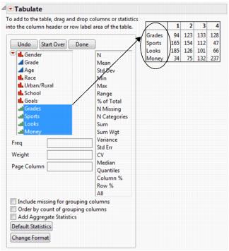
Notice that a single, combined table appears.
Tabulate the percentage of the one to four ratings of each category.
4. Drag Gender into the empty heading at left.
5. Drag % of Total above the numbered headings.
6. Drag All beside the number 4.
Figure 11.21 Gender, % of Total, and All Added to the Table
Break down the tabulation further by adding demographic data.
7. Drag Urban/Rural below the % of Total heading.
Figure 11.22 Urban/Rural Added to the Table
You can see that for boys in rural, suburban, and urban areas, sports are the most important factor for popularity. For girls in rural, suburban, and urban areas, looks are the most important factor for popularity.
Example Using a Page Column
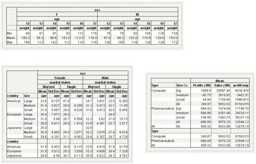
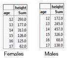
You have data containing height measurements for male and female students. You want to create a table that shows the mean height by the age of the students. Then you want to stratify your data by sex in different tables. To do so, add the stratification column as a page column, which will build the pages for each group. You want the table to look like Figure 11.23.
Figure 11.23 Mean Height of Students by Sex
1. Open the Big Class.jmp sample data table.
2. Select Analyze > Tabulate.
Since height is the variable you are examining, you want it to appear at the top of the table.
3. Click height and drag it into the Drop zone for columns.
You want the statistics by age, and you want age to appear on the side.
4. Click age and drag it into the blank cell next to the number 2502.0.
5. Click sex and drag it into Page Column.
F is selected, showing the mean heights for only females.
6. Click M to show the mean heights for only males. You can also click None Selected to select neither sex and show all values.
Figure 11.24 Using a Page Column
..................Content has been hidden....................
You can't read the all page of ebook, please click here login for view all page.