- Modeling algebraic expressions as data structures
- Writing code to analyze, transform, or evaluate algebraic expressions
- Finding the derivative of a function by manipulating the expression that defines it
- Writing a Python function to compute derivative formulas
- Using the SymPy library to compute integral formulas
If you followed all of the code examples and did all the exercises in chapter 8 and chapter 9, you already have a solid grasp of the two most important concepts in calculus: the derivative and the integral. First, you learned how to approximate the derivative of a function at a point by taking slopes of smaller and smaller secant lines. You then learned how to approximate an integral by estimating the area under a graph with skinny rectangles. Lastly, you learned how to do calculus with vectors by simply doing the relevant calculus operations in each coordinate.
It might seem like an audacious claim, but I really do hope to have given you the most important concepts you’d learn in a year-long college calculus class in just a few chapters of this book. Here’s the catch: because we’re working in Python, I’m skipping the most laborious piece of a traditional calculus course, which is doing a lot of formula manipulation by hand. This kind of work enables you to take the formula for a function like f(x) = x3 and figure out an exact formula for its derivative, f'(x). In this case, there’s a simple answer, f'(x) = 3x2, as shown in figure 10.1.

Figure 10.1 The derivative of the function f(x) = x3 has an exact formula, namely f'(x) = 3x2.
There are infinitely many formulas you might want to know the derivative of, and you can’t memorize derivatives for all of them, so what you end up doing in a calculus class is learning a small set of rules and how to systematically apply them to transform a function into its derivative. By and large, this isn’t that useful of a skill for a programmer. If you want to know the exact formula for a derivative, you can use a specialized tool called a computer algebra system to compute it for you.
10.1 Finding an exact derivative with a computer algebra system
One of the most popular computer algebra systems is called Mathematica, and you can use its engine for free online at a website called Wolfram Alpha (wolframalpha.com). In my experience, if you want an exact formula for a derivative for a program you’re writing, the best approach is to consult Wolfram Alpha. For instance, when we build a neural network in chapter 16, it will be useful to know the derivative of the function

To find a formula for the derivative of this function, you can simply go to wolframalpha.com and enter the formula in the input box (figure 10.2). Mathematica has its own syntax for mathematical formulas, but Wolfram Alpha is impressively forgiving and understands most simple formulas that you enter (even in Python syntax!).

Figure 10.2 Entering a function in the input box at wolframalpha.com
When you press Enter, the Mathematica engine powering Wolfram Alpha computes a number of facts about this function, including its derivative. If you scroll down, you’ll see a formula for the derivative of the function (figure 10.3).

Figure 10.3 Wolfram Alpha reports a formula for the derivative of the function.
For our function f(x), its instantaneous rate of change at any value of x is given by

If you understand the concept of a “derivative” and of an “instantaneous rate of change,” learning to punch formulas into Wolfram Alpha is a more important skill than any other single skill you’ll learn in a calculus class. I don’t mean to be cynical; there’s plenty to learn about the behavior of specific functions by taking their derivatives by hand. It’s just that in your life as a professional software developer, you’ll probably never need to figure out the formula for a derivative or integral when you have a free tool like Wolfram Alpha available.
That said, your inner nerd may be asking, “How does Wolfram Alpha do it?” It’s one thing to find a crude estimate of a derivative by taking approximate slopes of the graph at various points, but it’s another to produce an exact formula. Wolfram Alpha successfully interprets the formula you type in, transforms it with some algebraic manipulations, and outputs a new formula. This kind of approach, where you work with formulas themselves instead of numbers, is called symbolic programming.
The pragmatist in me wants to tell you to “just use Wolfram Alpha,” while the math enthusiast in me wants to teach you how to take derivatives and integrals by hand, so in this chapter I’m going to split the difference. We do some symbolic programming in Python to manipulate algebraic formulas directly and, ultimately, figure out the formulas for their derivatives. This gets you acquainted with the process of finding derivative formulas, while still letting the computer do most of the work for you.
10.1.1 Doing symbolic algebra in Python
Let me start by showing you how we’ll represent and manipulate formulas in Python. Say we have a mathematical function like
The usual way to represent it in Python is as follows:
from math import sin
def f(x):
    return (3*x**2 + x) * sin(x)
While this Python code makes it easy to evaluate the formula, it doesn’t give us a way to compute facts about the formula. For instance, we could ask
We can look at these questions and quickly decide that the answers are yes, yes, and no. There’s no simple, reliable way to write a Python program to answer these questions for us. For instance, it’s difficult, if not impossible, to write a function contains_division(f) that takes the function f and returns true if it uses the operation of division in its definition.
Here’s where this would come in handy. In order to invoke an algebraic rule, you need to know what operations are being applied and in what order. For instance, the function f(x) is a product of sin(x) with a sum, and there’s a well-known algebraic process for expanding a product of a sum as visualized in figure 10.4.

Figure 10.4 Because (3x2+x) sin(x) is a product of a sum, it can be expanded.
Our strategy is to model algebraic expressions as data structures rather than translating them directly to Python code, and then they’re more amenable to manipulation. Once we can manipulate functions symbolically, we can automate the rules of calculus.
Most functions expressed by simple formulas also have simple formulas for their derivatives. For instance, the derivative of x3 is 3x2, meaning at any value of x, the derivative of f(x) = x3 is given by 3x2. By the time we’re done in this chapter, you’ll be able to write a Python function that takes an algebraic expression and gives you an expression for its derivative. Our data structure for an algebraic formula will be able to represent variables, numbers, sums, differences, products, quotients, powers, and special functions like sine and cosine. If you think about it, we can represent a huge variety of different formulas with that handful of building blocks, and our derivative will work on all of them (figure 10.5).

Figure 10.5 A goal is to write a derivative function in Python that takes an expression for a function and returns an expression for its derivative.
We’ll get started by modeling expressions as data structures instead of functions in Python code. Then, to warm up, we can do some simple computations with the data structures to do things like plugging in numbers for variables or expanding products of sums. After that, I’ll teach you some of the rules for taking derivatives of formulas, and we’ll write our own derivative function and perform them automatically on our symbolic data structures.
10.2 Modeling algebraic expressions
Let’s focus on the function f(x) = (3x2 + x) sin(x) for a bit and see how we can break it down into pieces. This is a good example function because it contains a lot of different building blocks: a variable x, as well as numbers, addition, multiplication, a power, and a specially named function, sin(x). Once we have a strategy for breaking this function down into conceptual pieces, we can translate it into a Python data structure. This data structure is a symbolic representation of the function as opposed to a string representation like "(3*x**2 + x) * sin(x)".
A first observation is that f is an arbitrary name for this function. For instance, the right-hand side of this equation expands the same way regardless of what we call it. Because of this, we can focus only on the expression that defines the function, which in this case is (3x2 + x) sin(x). This is called an expression in contrast to an equation, which must contain an equals sign (=). An expression is a collection of mathematical symbols (numbers, letters, operations, and so on) combined in some valid ways. Our first goal, therefore, is to model these symbols and the valid means of composing this expression in Python.
10.2.1 Breaking an expression into pieces
We can start to model algebraic expressions by breaking them up into smaller expressions. There is only one meaningful way to break up the expression (3x2 + x) sin(x). Namely, it’s the product of (3x2 + x) and sin(x) as shown in figure 10.6.

Figure 10.6 A meaningful way to break up an algebraic expression into two smaller expressions
By contrast, we can’t split this expression around the plus sign. We could make sense of the expressions on either side of the plus sign if we tried, but the result is not equivalent to the original expression (figure 10.7).

Figure 10.7 It doesn’t make sense to split the expression up around the plus sign because the original expression is not the sum of 3x2 and x · sin(x).
If we look at the expression 3x2 + x, it can be broken up into a sum: 3x2 and x. Likewise, the conventional order of operations tells us that 3x2 is the product of 3 and x2, not 3x raised to the power of 2.
In this chapter, we’ll think of operations like multiplication and addition as ways to take two (or more) algebraic expressions and stick them together side by side to make a new, bigger algebraic expression. Likewise, operators are valid places to break up an existing algebraic expression into smaller ones.
In the terminology of functional programming, functions combining smaller objects into bigger ones like this are often called combinators. Here are some of the combinators implied in our expression:
-
x2 is a power: one expression x raised to the power of another expression 2.
-
The expression sin(x) is a function application. Given the expression sin and the expression x, we can build a new expression sin(x).
A variable x, a number 2, or a function named sin can’t be broken down further. To distinguish these from combinators, we call them elements. The lesson here is that while (3x2 + x) sin(x) is just a bunch of symbols printed on this page, the symbols are combined in certain ways to convey some mathematical meaning. To bring this concept home, we can visualize how this expression is built from its underlying elements.
10.2.2 Building an expression tree
The elements 3, x, 2, and sin, along with the combinators of adding, multiplying, raising to a power, and applying a function are sufficient to rebuild the whole of the expression (3x2 + x) sin(x). Let’s go through the steps and draw the structure we’ll end up building. One of the first constructions we can put together is x2, which combines x and 2 with the power combinator (figure 10.8).

Figure 10.8 Combining x and 2 with the power combinator to represent the bigger expression x2
A good next step is to combine x2 with the number 3 via the product combinator to get the expression 3x2 (figure 10.9).

Figure 10.9 Combining the number 3 with a power to model the product 3x2
This construction is two layers deep: one expression that inputs to the product combinator is itself a combinator. As we add more of the terms of the expression, it gets even deeper. The next step is adding the element x to 3x2 using the sum combinator (figure 10.10), which represents the operation of addition.

Figure 10.10 Combining the expression 3x2 with the element x and the sum combinator to get 3x2 + x
Finally, we need to use the function application combinator to apply sin to x and then the product combinator to combine sin(x) with what we’ve built thus far (figure 10.11).
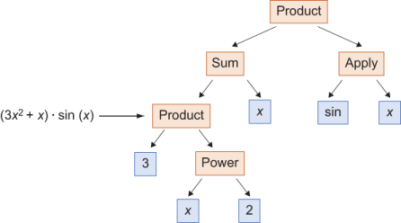
Figure 10.11 A completed picture showing how to build (3x2 + x) sin(x) from elements and combinators
You may recognize the structure we’ve built as a tree. The root of the tree is the product combinator with two branches coming out of it: Sum and Apply. Each combinator appearing further down the tree adds additional branches, until you reach the elements that are leaves and have no branches. Any algebraic expression built with numbers, variables, and named functions as elements and operations that are combinators correspond to a distinctive tree that reveals its structure. The next thing we can do is to build the same tree in Python.
10.2.3 Translating the expression tree to Python
When we’ve built this tree in Python, we’ll have achieved our goal of representing the expression as a data structure. I’ll use Python classes covered in appendix B to represent each kind of element and each combinator. As we go, we’ll revise these classes to give them more and more functionality. You can follow the walk-through Jupyter notebook for chapter 10 if you want to follow the text, or you can skip to a more complete implementation in the Python script file expressions.py.
In our implementation, we model combinators as containers that hold all of their inputs. For instance, a power x to the 2, or x2, has two pieces of data: the base x and the power 2. Here’s a Python class that’s designed to represent a power expression:
class Power():
    def __init__(self,base,exponent):
        self.base = base
        self.exponent = exponent
We could then write Power("x",2) to represent the expression x2. But rather than using raw strings and numbers, I’ll create special classes to represent numbers and variables. For example,
class Number():
    def __init__(self,number):
        self.number = number

class Variable():
    def __init__(self,symbol):
        self.symbol = symbol
This might seem like unnecessary overhead, but it will be useful to be able to distinguish Variable("x"), which means the letter x considered as a variable from the string "x", which is merely a string. Using these three classes, we can model the expression x2 as
Power(Variable("x"),Number(2))
Each of our combinators can be implemented as an appropriately named class that stores the data of whatever expressions it combines. For instance, a product combinator can be a class that stores two expressions that are meant to be multiplied together:
class Product():
    def __init__(self, exp1, exp2):
        self.exp1 = exp1
        self.exp2 = exp2
The product 3x2 can be expressed using this combinator:
Product(Number(3),Power(Variable("x"),Number(2)))
After introducing the rest of the classes we need, we can model the original expression as well as an infinite list of other possibilities. (Note that we allow any number of input expressions for the Sum combinator, and we could have done this for the Product combinator as well. I restricted the Product combinator to two inputs to keep our code simpler when we start calculating derivatives in section 10.3.)
class Sum():
    def __init__(self, *exps):            ❶
        self.exps = exps

class Function():                         ❷
    def __init__(self,name):
        self.name = name

class Apply():                            ❸
    def __init__(self,function,argument):
        self.function = function
        self.argument = argument

f_expression = Product(>                  ❹
               Sum(
                   Product(
                       Number(3),
                       Power(
                           Variable("x"),
                           Number(2))),
                   Variable("x")),
               Apply(
                   Function("sin"),
                   Variable("x")))
❶ Allows a Sum of any number of terms so we can add two or more expressions together
❷ Stores a string that is the function’s name (like “sin”)
❸ Stores a function and the argument it is applied to
❹ I use extra whitespace to make the structure of the expression clearer to see.
This is a faithful representation of the original expression (3x2 + x) sin(x). By that I mean, we could look at this Python object and see that it describes the algebraic expression and not a different one. For another expression like
Apply(Function("cos"),Sum(Power(Variable("x"),Number("3")), Number(−5)))
we can read it carefully and see that it represents a different expression: cos(x3 + −5). In the exercises that follow, you can practice translating some algebraic expressions to Python and vice versa. You’ll see it can be tedious to type out the whole representation of an expression. The good news is that once you get it encoded in Python, the manual work is over. In the next section, we see how to write Python functions to automatically work with our expressions.
10.2.4 Exercises
|
|

from math import log
def f(y,z):
    return log(y**z)
Apply(Function("ln"), Power(Variable("y"), Variable("z")))
|
|
class Quotient():
    def __init__(self,numerator,denominator):
        self.numerator = numerator
        self.denominator = denominator
Quotient(Sum(Variable("a"),Variable("b")),Number(2))
|

class Difference():
    def __init__(self,exp1,exp2):
        self.exp1 = exp1
        self.exp2 = exp2
Difference(
    Power(Variable('b'),Number(2)),
    Product(Number(4),Product(Variable('a'), Variable('c'))))
|
class Negative():
    def __init__(self,exp):
        self.exp = exp
Negative(Sum(Power(Variable("x"),Number(2)),Variable("y")))
|
|
A = Variable('a')
B = Variable('b')
C = Variable('c')
Sqrt = Function('sqrt')
Quotient(
    Sum(
        Negative(B),
        Apply(
            Sqrt,
            Difference(
                Power(B,Number(2)),
                Product(Number(4), Product(A,C))))),
    Product(Number(2), A))
|

10.3 Putting a symbolic expression to work
For the function we’ve studied so far, f(x) = (3x2 + x) sin(x), we wrote a Python function that computes it:
def f(x):
    return (3*x**2 + x)*sin(x)
As an entity in Python, this function is only good for one thing: returning an output value for a given input value x. The value f in Python does not make it particularly easy to programmatically answer the questions we asked at the beginning of the chapter: whether f depends on its input, whether f contains a trigonometric function, or what the body of f would look like if it were expanded algebraically. In this section, we see that once we translate the expression into a Python data structure built from elements and combinators, we can answer all of these questions and more!
10.3.1 Finding all the variables in an expression
Let’s write a function that takes an expression and returns a list of distinct variables that appear in it. For instance, h(z) = 2z + 3 is defined using the input variable z, while the definition of g(x) = 7 contains no variables. We can write a Python function, distinct_variables, that takes an expression (meaning any of our elements or combinators) and returns a Python set containing the variables.
If our expression is an element, like z or 7, the answer is clear. An expression that is just a variable contains one distinct variable, while an expression that is just a number contains no variables at all. We expect our function to behave accordingly:
>>> distinct_variables(Variable("z"))
{'z'}
>>> distinct_variables(Number(3))
set()
The situation is more complicated when the expression is built from some combinators like y · z + xz . It’s easy for a human to read all the variables, y, z, and x, but how do we extract these from the expression in Python? This is actually a Sum combinator representing the sum of y · z and xz . The first expression in the sum contains y and z, while the second has x and z. The sum then contains all of the variables in these two expressions.
This suggests we should use a recursive solution: the distinct_variables for a combinator are the collected distinct_variables for each of the expressions it contains. The end of the line has the variables and numbers, which obviously contain either one or zero variables. To implement the distinct_variables function, we need to handle the case of every element and combinator that make up a valid expression:
def distinct_variables(exp):
    if isinstance(exp, Variable):
        return set(exp.symbol)
    elif isinstance(exp, Number):
        return set()
    elif isinstance(exp, Sum):
        return set().union(*[distinct_variables(exp) for exp in exp.exps])
    elif isinstance(exp, Product):
        return distinct_variables(exp.exp1).union(distinct_variables(exp.exp2))
    elif isinstance(exp, Power):
        return distinct_variables(exp.base).union(distinct_variables(exp.exponent))
    elif isinstance(exp, Apply):
        return distinct_variables(exp.argument)
    else:
        raise TypeError("Not a valid expression.")
This code looks hairy, but it is just a long if/else statement with one line for each possible element or combinator. Arguably, it would be better coding style to add a distinct_variables method to each element and combinator class, but that makes it harder to see the logic in a single code listing. As expected, our f_expression contains only the variable x :
>>> distinct_variables(f_expression)
{'x'}
If you’re familiar with the tree data structure, you’ll recognize this as a recursive traversal of the expression tree. By the time this function completes, it has called distinct_variables on every expression contained in the target expression, which are all of the nodes in the tree. That ensures that we see every variable and that we get the correct answers that we expect. In the exercises at the end of this section, you can use a similar approach to find all of the numbers or all of the functions.
10.3.2 Evaluating an expression
Now, we’ve got two representations of the same mathematical function f(x ). One is the Python function f, which is good for evaluating the function at a given input value of x. The new one is this tree data structure that describes the structure of the expression defining f(x). It turns out the latter representation has the best of both worlds; we can use it to evaluate f(x) as well, with only a little more work.
Mechanically, evaluating a function f(x) at, say, x = 5 means plugging in the value of 5 for x everywhere and then doing the arithmetic to find the result. If the expression were just f(x) = x, plugging in x = 5 would tell us f(5) = 5. Another simple example would be g(x) = 7, where plugging in 5 in place of x has no effect; there are no appearances of x on the right-hand side, so the result of g(5) is just 7.
The code to evaluate an expression in Python is similar to the code we just wrote to find all variables. Instead of looking at the set of variables that appear in each subexpression, we need to evaluate each subexpression, then the combinators tell us how to combine these results to get the value of the whole expression.
The starting data we need is what values to plug-in and which variables these replace. An expression with two different variables like z(x, y) = 2xy3 will need two values to get a result; for instance, x = 3 and y = 2. In computer science terminology, these are called variable bindings. With these, we can evaluate the subexpression y3 as (2)3, which equals 8. Another subexpression is 2x, which evaluates to 2 · (3) = 6. These two are combined with the Product combinator, so the value of the whole expression is the product of 6 and 8, or 48.
As we translate this procedure into Python code, I’m going to show you a slightly different style than in the previous example. Rather than having a separate evaluate function, we can add an evaluate method to each class representing an expression. To enforce this, we can create an abstract Expression base class with an abstract evaluate method and have each kind of expression inherit from it. If you need a review of abstract base classes in Python, take a moment to review the work we did with the Vector class in chapter 6 or the overview in appendix B. Here’s an Expression base class, complete with an evaluate method:
from abc import ABC, abstractmethod

class Expression(ABC):
    @abstractmethod
    def evaluate(self, **bindings):
        pass
Because an expression can contain more than one variable, I set it up so you can pass in the variable bindings as keyword arguments. For instance, the bindings {"x":3,"y":2} mean substitute 3 for x and 2 for y. This gives us some nice syntactic sugar when evaluating an expression. If z represents the expression 2xy3, then once we’re done, we’ll be able to execute the following:
>>> z.evaluate(x=3,y=2)
48
So far, we’ve only an abstract class. Now we need to have all of our expression classes inherit from Expression. For example, a Number instance is a valid expression as a number on its own, like 7. Regardless of the variable bindings provided, a number evaluates to itself:
class Number(Expression):
    def __init__(self,number):
        self.number = number
    def evaluate(self, **bindings):
        return self.number
For instance, evaluating Number(7).evaluate(x=3,y=6,q=−15), or any other evaluation for that matter, returns the underlying number 7.
Handling variables is also simple. If we’re looking at the expression Variable("x"), we only need to consult the bindings and see what number the variable x is set to. When we’re done, we should be able to run Variable("x").evaluate(x=5) and get 5 as a result. If we can’t find a binding for x, then we can’t complete the evaluation, and we need to raise an exception. Here’s the updated definition of the Variable class:
class Variable(Expression):
    def __init__(self,symbol):
        self.symbol = symbol
    def evaluate(self, **bindings):
        try:
            return bindings[self.symbol]
        except:
            raise KeyError("Variable '{}' is not bound.".format(self.symbol))
With these elements handled, we need to turn our attention to the combinators. (Note that we won’t consider a Function object an Expression on its own because a function like sine is not a standalone expression. It can only be evaluated when it’s given an argument in the context of an Apply combinator.) For a combinator like Product, the rule to evaluate it is simple: evaluate both expressions contained in the product and then multiply the results together. No substitution needs to be performed in the product, but we’ll pass the bindings along to both subexpressions in case either contains a Variable :
class Product(Expression):
    def __init__(self, exp1, exp2):
        self.exp1 = exp1
        self.exp2 = exp2
    def evaluate(self, **bindings):
        return self.exp1.evaluate(**bindings) * self.exp2.evaluate(**bindings)
With these three classes updated with evaluate methods, we can now evaluate any expression built from variables, numbers, and products. For instance,
>>> Product(Variable("x"), Variable("y")).evaluate(x=2,y=5)
10
Similarly, we can add an evaluate method to the Sum, Power, Difference, or Quotient combinators (as well as any other combinators you may have created as exercises). Once we evaluate their subexpressions, the name of the combinator tells us which operation we can use to get the overall result.
The Apply combinator works a bit differently, so it deserves some special attention. We need to dynamically look at a function name like sin or sqrt and figure out how to compute its value. There are a few possible ways to do this, but I chose keeping a dictionary of known functions as data on the Apply class. As a first pass, we can make our evaluator aware of three named functions:
_function_bindings = {
    "sin": math.sin,
    "cos": math.cos,
    "ln": math.log
}
class Apply(Expression):
    def __init__(self,function,argument):
        self.function = function
        self.argument = argument
    def evaluate(self, **bindings):
        return _function_bindings[self.function.name](self.argument.evaluate(**bindings))
You can practice writing the rest of the evaluate methods yourself or find them in the source code for this book. Once you get all of them fully implemented, you’ll be able to evaluate our f_expression from section 10.1.3:
>>>  f_expression.evaluate(x=5)
−76.71394197305108
The result here isn’t important, only the fact that it’s the same as what the ordinary Python function f(x) gives us:
>>> xf(5)
−76.71394197305108
Equipped with the evaluate function, our Expression objects can do the same work as their corresponding ordinary Python functions.
10.3.3 Expanding an expression
There are many other things we can do with our expression data structures. In the exercises, you can try your hand at building a few more Python functions that manipulate expressions in different ways. I’ll show you one more example for now, which I mentioned at the beginning of this chapter: expanding an expression. What I mean by this is taking any product or power of sums and carrying it out.
The relevant rule of algebra is the distributive property of sums and products. This rule says that a product of the form (a + b) · c is equal to ac + bc and, similarly, that x(y + z) = xy + xz. For instance, our expression (3x2 + x) sin(x) is equal to 3x2 sin(x) + x sin(x), which is called the expanded form of the first product. You can use this rule several times to expand more complicated expressions, for instance:
(x + y)3 = (x + y)(x + y)(x + y)
= x(x + y)(x + y) + y(x + y)(x + y)
= x2(x + y) + xy(x + y) + yx(x + y) + y2(x + y)
= x3 + x2y + x2y + xy2 + yx2 + y2x + y2x + y3
= x3 + 3x2y + 3y2x + y3
As you can see, expanding a short expression like (x + y)3 can be a lot of writing. In addition to expanding this expression, I also simplified the result a bit, rewriting some products that would have looked like xyx or xxy as x2 y, for instance. This is possible because order does not matter in multiplication. Then I further simplified by combining like terms, noting that there were three summed copies each of x2 y and y2 x and grouping those together into 3x2 y and 3y2 x. In the following example, we only look at how to do the expanding; you can implement the simplification as an exercise.
We can start by adding an abstract expand method to the Expression base class:
class Expression(ABC):
    ...
    @abstractmethod
    def expand(self):
        pass
If an expression is a variable or number, it is already expanded. For these cases, the expand method returns the object itself. For instance,
class Number(Expression):
    ...
    def expand(self):
        return self
Sums are already considered to be expanded expressions, but the individual terms of a sum cannot be expanded. For example, 5 + a(x + y) is a sum in which the first term 5 is fully expanded, but the second term a(x + y) is not. To expand a sum, we need to expand each of the terms and sum them:
class Sum(Expression):
    ...
    def expand(self):
        return Sum(*[exp.expand() for exp in self.exps])
The same procedure works for function application. We can’t expand the Apply function itself, but we can expand its arguments. This would expand an expression like sin(x(y + z)) to sin(xy + xz):
class Apply(Expression):
    ...
    def expand(self):
        return Apply(self.function, self.argument.expand())
The real work comes when we expand products or powers, where the structure of the expression changes completely. As an example, a(b + c) is a product of a variable with a sum of two variables, while its expanded form is ab + ac, the sum of two products of two variables each. To implement the distributive law, we have to handle three cases: the first term of the product might be a sum, the second term might be a sum, or neither of them might be sums. In the latter case, no expanding is necessary:
class Product(Expression):
    ...
    def expand(self):
        expanded1 = self.exp1.expand()                 ❶
        expanded2 = self.exp2.expand()
        if isinstance(expanded1, Sum):                 ❷
            return Sum(*[Product(e,expanded2).expand()
                         for e in expanded1.exps])
        elif isinstance(expanded2, Sum):               ❸
            return Sum(*[Product(expanded1,e)
                         for e in expanded2.exps])
        else:
            return Product(expanded1,expanded2)        ❹
❶ Expands both terms of the product
❷ If the first term of the product is a Sum, it takes the product with each of its terms multiplied by the second term of the product, then calls expand on the result in case the second term of the product is also a Sum.
❸ If the second term of the product is a Sum, it multiplies each of its terms by the first term of the product.
❹ Otherwise, neither term is a Sum, and the distributive property doesn’t need to be invoked.
With all of these methods implemented, we can test the expand function. With an appropriate implementation of __repr__(see the exercises), we can see a string representation of the results clearly in Jupyter or in an interactive Python session. It correctly expands (a + b) (x + y) to ax + ay + bx + by :
Y = Variable('y')
Z = Variable('z')
A = Variable('a')
B = Variable('b')
>>> Product(Sum(A,B),Sum(Y,Z))
Product(Sum(Variable("a"),Variable("b")),Sum(Variable("x"),Variable("y")))
>>> Product(Sum(A,B),Sum(Y,Z)).expand()
Sum(Sum(Product(Variable("a"),Variable("y")),Product(Variable("a"),
Variable("z"))),Sum(Product(Variable("b"),Variable("y")),
Product(Variable("b"),Variable("z"))))
And our expression, (3x2 + x) sin(x), expands correctly to 3x2 sin(x) + x sin(x):
>>> f_expression.expand()
Sum(Product(Product(3,Power(Variable("x"),2)),Apply(Function("sin"),Variable("x"))),Product(Variable("x"),Apply(Function("sin"),Variable("x"))))
At this point, we’ve written some Python functions that really do algebra for us, not just arithmetic. There are a lot of exciting applications of this type of programming (called symbolic programming, or more specifically, computer algebra), and we can’t afford to cover all of them in this book. You should try your hand at a few of the following exercises and then we move on to our most important example: finding the formulas for derivatives.
10.3.4 Exercises
def contains(exp, var):
    if isinstance(exp, Variable):
        return exp.symbol == var.symbol
    elif isinstance(exp, Number):
        return False
    elif isinstance(exp, Sum):
        return any([contains(e,var) for e in exp.exps])
    elif isinstance(exp, Product):
        return contains(exp.exp1,var) or contains(exp.exp2,var)
    elif isinstance(exp, Power):
        return contains(exp.base, var) or contains(exp.exponent, var)
    elif isinstance(exp, Apply):
        return contains(exp.argument, var)
    else:
        raise TypeError("Not a valid expression.")
|
def distinct_functions(exp):
    if isinstance(exp, Variable):
        return set()
    elif isinstance(exp, Number):
        return set()
    elif isinstance(exp, Sum):
        return set().union(*[distinct_functions(exp) for exp in exp.exps])
    elif isinstance(exp, Product):
        return distinct_functions(exp.exp1).union(distinct_functions(exp.exp2))
    elif isinstance(exp, Power):
        return distinct_functions(exp.base).union(distinct_functions(exp.exponent))
    elif isinstance(exp, Apply):
        return set([exp.function.name]).union(distinct_functions(exp.argument))
    else:
        raise TypeError("Not a valid expression.")
|
def contains_sum(exp):
    if isinstance(exp, Variable):
        return False
    elif isinstance(exp, Number):
        return False
    elif isinstance(exp, Sum):
        return True
    elif isinstance(exp, Product):
        return contains_sum(exp.exp1) or contains_sum(exp.exp2)
    elif isinstance(exp, Power):
        return contains_sum(exp.base) or contains_sum(exp.exponent)
    elif isinstance(exp, Apply):
        return contains_sum(exp.argument)
    else:
        raise TypeError("Not a valid expression.")
|
|
|

>>> Power(Variable("x"),Number(2))._python_expr()
'(x) ** (2)'
>>> Power(Variable("x"),Number(2)).python_function(x=3)
9
|
10.4 Finding the derivative of a function
It might not seem obvious, but there is often a clean algebraic formula for the derivative of a function. For instance, if f(x) = x3, then its derivative f'(x), which measures the instantaneous rate of change in f at any point x, is given by f'(x) = 3x2. If you know a formula like this, you can get an exact result such as f'(2) = 12 without the numerical issues associated with using small secant lines.
If you took calculus in high school or college, chances are you spent a lot of time learning and practicing how to find formulas for derivatives. It’s a straightforward task that doesn’t require much creativity, and it can be tedious. That’s why we’ll briefly spend time covering the rules and then focus on having Python do the rest of the work for us.
10.4.1 Derivatives of powers
Without knowing any calculus, you can find the derivative of a linear function of the form f(x) = mx + b. The slope of any secant on this line, no matter how small, is the same as the slope of the line m ; therefore, f'(x) doesn’t depend on x. Specifically, we can say f'(x) = m. This makes sense: a linear function f(x) changes at a constant rate with respect to its input x, so its derivative is a constant function. Also, the constant b has no effect on the slope of the line, so it doesn’t appear in the derivative (figure 10.12).

Figure 10.12 The derivative of a linear function is a constant function.
It turns out the derivative of a quadratic function is a linear function. For instance, q(x) = x2 has derivative q'(x) = 2x. This also makes sense if you plot the graph of q(x). The slope of q(x) starts negative, increases, and eventually becomes positive after x = 0. The function q'(x) = 2x agrees with this qualitative description.
As another example, I showed you that x3 has derivative 3x2. All of these facts are special cases of a general rule: when you take the derivative of a function f(x), which is a power of x, you get back a function that is one lower power. Specifically, figure 10.13 shows the derivative of a function of the form axn is naxn −1.

Figure 10.13 A general rule for derivatives of powers: taking the derivative of a function f(x), a power of x, returns a function that is one power lower.
Let’s break this down for a specific example. If g(x) = 5x4, then this has the form axn with a = 5 and n = 4. The derivative is naxn −1, which becomes 4 · 5 · x4−1 = 20x3. Like any other derivative we’ve covered in this chapter, you can double-check this by plotting it alongside the result from our numerical derivative function from chapter 9. The graphs should coincide exactly.
A linear function like f(x) is a power of x : f(x) = mx1. The power rule applies here as well: mx1 has a derivative 1 · mx0 because x0 = 1. By geometric considerations, adding a constant b does not change the derivative; it moves the graph up and down, but it doesn’t change the slope.
10.4.2 Derivatives of transformed functions
Adding a constant to a function never changes its derivative. For instance, the derivative of x100 is 100x99, and the derivative of x100 − π is also 100x99. But some modifications of a function do change the derivative. For example, if you put a negative sign in front of a function, the graph flips upside down and so does the graph of any secant line. If the slope of the secant line is m before the flip, it is − m after; the change in x is the same as before, but the change in y = f(x) is now in the opposite direction (figure 10.14).

Figure 10.14 For any secant line on f(x), the secant line on the same x interval of -f(x) has the opposite slope.
Because derivatives are determined by the slopes of secant lines, the derivative of a negative function -f(−x) is equal to the negative derivative -f'(x). This agrees with the formula we’ve already seen: if f(x) = −5x2 then a = −5 and f'(x) = −10x(as compared to 5x2, which has the derivative +10x). Another way to put this is that if you multiply a function by −1, then its derivative is multiplied by −1 as well.
The same turns out to be true for any constant. If you multiply f(x) by 4 to get 4f(x), figure 10.15 shows that this new function is four times steeper at every point and, therefore, its derivative is 4f'(x).

Figure 10.15 Multiplying a function by 4 makes every secant line four times steeper.
This agrees with the power rule for derivatives I showed you. Knowing the derivative of x2 is 2x, you also know that the derivative of 10x2 is 20x, the derivative of −3x2 is −6x, and so on. We haven’t covered it yet, but if I tell you the derivative of sin(x) is cos(x), you’ll know right away that the derivative of 1.5 · sin(x) is 1.5 · cos(x).
A final transformation that’s important is adding two functions together. If you look at the graph of f(x) + g(x) for any pair of functions f and g in figure 10.16, the vertical change for any secant line is the sum of the vertical changes in f and g on that interval.
When we’re working with formulas, we can take the derivative of each term in a sum independently. If we know that the derivative of x2 is 2x, and the derivative of x3 is 3x2, then the derivative of x2 + x3 is 2x + 3x2. This rule gives a more precise reason why the derivative of mx + b is m ; the derivatives of the terms are m and 0, respectively, so the derivative of the whole formula is m + 0 = m.

Figure 10.16 The vertical change in f(x) on some x interval is the sum of the vertical change in f(x) and in g(x) on that interval.
10.4.3 Derivatives of some special functions
There are plenty of functions that can’t be written in the form axn or even as a sum of terms of this form. For example, trigonometric functions, exponential functions, and logarithms all need to be covered separately. In a calculus class, you learn how to figure out the derivatives of these functions from scratch, but that’s beyond the scope of this book. My goal is to show you how to take derivatives so that when you meet them in the wild, you’ll be able to solve the problem at hand. To that end, I give you a quick list of some other important derivative rules (table 10.1).
Table 10.1 Some basic derivatives (continued)
You can use this table along with the previous rules to figure out more complicated derivatives. For instance, let f(x) = 6x + 2 sin(x) + 5 ex. The derivative of the first term is 6, by the power rule from section 10.4.1. The second term contains sin(x), whose derivative is cos(x), and the factor of two doubles the result, giving us 2 cos(x). Finally, ex is its own derivative (a very special case!), so the derivative of 5 ex is 5 ex. All together the derivative is f'(x) = 6 + 2 cos(x) + 5 ex.
You have to be careful to only use the rules we’ve covered so far: the power law (section 10.4.1), the rules in the table 10.1, and the rules for sums and scalar multiples. If your function is g(x) = sin(sin(x)), you might be tempted to write g'(x) = cos(cos(x)), substituting in the derivative for sine in both of its appearances. But this is not correct! Nor can you infer that the derivative of the product ex cos(x) is − ex sin(x). When functions are combined in other ways than addition and subtraction, we need new rules to take their derivatives.
10.4.4 Derivatives of products and compositions
Let’s look at a product like f(x) = x2 sin(x). This function can be written as a product of two other functions: f(x) = g(x) · h(x), where g(x) = x2 and h(x) = sin(x). As I just warned you, f'(x) is not equal to g'(x) · h'(x) here. Fortunately, there’s another formula that is true, and it’s called the product rule for derivatives.
The product rule If f(x) can be written as the product of two other functions g and h as in f(x) = g(x) · h(x), then the derivative of f(x) is given by:
f'(x) = g'(x) · h(x) + g(x) · h'(x)
Let’s practice applying this rule to f(x) = x2 sin(x). In this case, g(x) = x2 and h(x) = sin(x), so g'(x) = 2x and h'(x) = cos(x) as I showed you previously. Plugging these into the product rule formula f'(x) = g'(x) · h(x) + g(x) · h'(x), we get f'(x) = 2x sin(x) + x2 cos(x). That’s all there is to it!
You can see that this product rule is compatible with the power rule from section 10.4.1. If you rewrite x2 as the product of x · x, the product rule tells you its derivative is 1 · x + x · 1 = 2x.
Another important rule tells us how to take derivatives of composed functions like ln(cos(x)). This function has the form f(x) = g(h(x)), where g(x) = ln(x) and h(x) = cos(x). We can’t just plug in the derivatives where we see the functions, getting −1/sin(x); the answer is a bit more complicated. The formula for the derivative of a function of the form f(x) = g(h(x)) is called the chain rule.
The chain rule If f(x)is a composition of two functions, meaning it can be written in the form f(x) = g(h(x)) for some functions g and h, then the derivative of f is given by:
In our case, g'(x) = 1/x and h'(x) = −sin(x) both read from table 10.1. Then plugging into the chain rule formula, we get the result:

You might remember that sin(x)/cos(x) = tan(x), so we could write even more concisely that the derivative of ln(cos(x)) = tan(x). I’ll give you a few more opportunities to practice the product and chain rule in the exercises, and you can also turn to any calculus book for abundant examples of calculating derivatives. You don’t need to take my word for these derivative rules; you should get a result that looks the same if you find a formula for the derivative or if you use the derivative function from chapter 9. In the next section, I’ll show you how to turn the rules for derivatives into code.
10.4.5 Exercises
def p(x):
    return x**5
plot_function(derivative(p), 0, 1)
plot_function(lambda x: 5*x**4, 0, 1)
|

|
|


|
|


|
|

10.5 Taking derivatives automatically
Even though I taught you only a few rules for taking derivatives, you’re now prepared to handle any of an infinite collection of possible functions. As long as a function is built from sums, products, powers, compositions, trigonometric functions, and exponential functions, you are equipped to figure out its derivative using the chain rule, product rule, and so on.
This parallels the approach we used to build algebraic expressions in Python. Even though there are infinitely many possibilities, they are all formed from the same set of building blocks and a handful of predefined ways to assemble them together. To take derivatives automatically, we need to match each case of a representable expression, be it an element or combinator, with the appropriate rule for taking its derivative. The end result is a Python function that takes one expression and returns a new expression representing its derivative.
10.5.1 Implementing a derivative method for expressions
Once again, we can implement the derivative function as a method on each of the Expression classes. To enforce that they all have this method, we can add an abstract method to the abstract base class:
class Expression(ABC):
    ...
    @abstractmethod
    def derivative(self,var):
        pass
The method needs to take a parameter, var, indicating which variable we’re taking a derivative with respect to. For instance, f(y) = y2 would need a derivative taken with respect to y. As a trickier example, we’ve worked with expressions like axn, where a and n represent constants and only x is the variable. From this perspective, the derivative is naxn −1. However, if we think of this instead as a function of a, as in f(a) = axn, the derivative is xn −1, a constant to a constant power. We get yet another result if we consider it a function of n : if f(n) = axn, then f'(n) = a ln(n) xn . To avoid confusion, we’ll consider all expressions as functions of the variable x in the following discussion.
As usual, our easiest examples are the elements: Number and Variable objects. For Number, the derivative is always the expression 0, regardless of the variable passed in:
class Number(Expression):
    ...
    def derivative(self,var):
        return Number(0)
If we’re taking the derivative of f(x) = x, the result is f'(x) = 1, which is the slope of the line. Taking the derivative of f(x) = c should give us 0 as c represents a constant here, rather than the argument of the function f . For that reason, the derivative of a variable is 1 only if it’s the variable we’re taking the derivative with respect to; otherwise, the derivative is 0:
class Variable(Expression):
    ...
    def derivative(self, var):
        if self.symbol == var.symbol:
            return Number(1)
        else:
            return Number(0)
The easiest combinator to take derivatives of is Sum; the derivative of a Sum function is just the sum of the derivatives of its terms:
class Sum(Expression):
    ...
    def derivative(self, var):
        return Sum(*[exp.derivative(var) for exp in self.exps])
With these methods implemented, we can do some basic examples. For instance, the expression Sum(Variable("x"),Variable("c"),Number(1)) represents x + c + 1, and thinking of that as a function of x, we can take its derivative with respect to x :
>>> Sum(Variable("x"),Variable("c"),Number(1)).derivative(Variable("x"))
Sum(Number(1),Number(0),Number(0))
This correctly reports the derivative of x + c + 1 with respect to x as 1 + 0 + 0, which is equal to 1. This is a clunky way to report the result, but at least we got it right.
I encourage you to do the mini-project for writing a simplify method that gets rid of extraneous terms, like added zeros. We could add some logic to simplify expressions as we compute the derivatives, but it’s better to separate our concerns and focus on getting the derivative right for now. Keeping that in mind, let’s cover the rest of the combinators.
10.5.2 Implementing the product rule and chain rule
The product rule turns out to be the easiest of the remaining combinators to implement. Given the two expressions that make up a product, the derivative of the product is defined in terms of those expressions and their derivatives. Remember, if the product is g(x) · h(x), the derivative is g'(x) · h(x) + g(x) · h'(x). That translates to the following code, which returns the result as the sum of two products:
class Product(Expression):
    ...
    def derivative(self,var):
        return Sum(
            Product(self.exp1.derivative(var), self.exp2),
            Product(self.exp1, self.exp2.derivative(var)))
Again, this gives us correct (albeit unsimplified) results. For instance, the derivative of cx with respect to x is
>>> Product(Variable("c"),Variable("x")).derivative(Variable("x"))
Sum(Product(Number(0),Variable("x")),Product(Variable("c"),Number(1)))
That result represents 0 · x + c · 1, which is, of course, c.
Now we’ve got the Sum and Product combinators handled, so let’s look at Apply. To handle a function application like sin(x2), we need to encode both the derivative of the sine function and the use of the chain rule because of the x2 inside the parentheses.
First, let’s encode the derivatives of some of the special functions in terms of a placeholder variable unlikely to be confused with any we use in practice. The derivatives are stored as a dictionary mapping from function names to expressions giving their derivatives:
_var = Variable('placeholder variable')                       ❶

_derivatives = {
    "sin": Apply(Function("cos"), _var),                      ❷
    "cos": Product(Number(−1), Apply(Function("sin"), _var)),
    "ln": Quotient(Number(1), _var)
}
❶ Creates a placeholder variable designed so that it’s not confused with any symbol (like x or y) that we might actually use
❷ Records that the derivative of sine is cosine, with cosine expressed as an expression using the placeholder variable
The next step is to add the derivative method to the Apply class, looking up the correct derivative from the _derivatives dictionary and appropriately applying the chain rule. Remember that the derivative of g(h(x)) is h'(x) · g'(h(x)). If, for example, we’re looking at sin(x2), then g(x) = sin(x) and h(x) = x2. We first go to the dictionary to get the derivative of sin, which we get back as cos with a placeholder value. We need to plug in h(x) = x2 for the placeholder to get the g'(h(x)) term from the chain rule. This requires a substitute function, which replaces all instances of a variable with an expression (a mini-project from earlier in the chapter). If you didn’t do that mini-project, you can see the implementation in the source code. The derivative method for Apply looks like this:
class Apply(Expression):
    ...
    def derivative(self, var):
        return Product(
                self.argument.derivative(var),                    ❶
                _derivatives[self.function.name].substitute(_var, self.argument))                                                   ❷
❶ Returns h'(x) in h'(x) · g'(h(x)) of the chain rule formula
❷ This is the g'(h(x)) of the chain rule formula, where the _derivatives dictionary looks up g' and h(x) is substituted in.
For sin(x2), for example, we have
>>> Apply(Function("sin"),Power(Variable("x"),Number(2))).derivative(x)
Product(Product(Number(2),Power(Variable("x"),Number(1))),Apply(Function("cos"),Power(Variable("x"),Number(2))))
Literally, that result translates to (2x1) · cos(x2), which is a correct application of the chain rule.
10.5.3 Implementing the power rule
The last kind of expression we need to handle is the Power combinator. There are actually three derivative rules we need to include in the derivative method for the Power class. The first is the rule I called the power rule, which tells us that xn has derivative nxn −1, when n is a constant. The second is the derivative of the function ax, where the base, a, is assumed to be constant while the exponent changes. This function has the derivative ln(a) · ax with respect to x.
Finally, we need to handle the chain rule here because there could be an expression involved in either the base or the exponent, like sin(x)8 or 15cos(x). There’s yet another case where both the base and the exponent are variables like nx or ln(x)sin(x). In all my years taking derivatives, I’ve never seen a real application where this case comes up, so I’ll skip it and raise an exception instead.
Because xn , g(x)n, ax , and ag(x) are all represented in Python in the form Power(expression1, expression2), we have to do some checks to find out what rule to use. If the exponent is a number, we use the xn rule, but if the base is a number, we use the ax rule. In both cases, I use the chain rule by default. After all, xn is a special case of f(x)n, where f(x) = x. Here’s what the code looks like:
class Power(Expression):
    ...
    def derivative(self,var):
        if isinstance(self.exponent, Number):                            ❶
            power_rule = Product(
                    Number(self.exponent.number),
                    Power(self.base, Number(self.exponent.number − 1)))
            return Product(self.base.derivative(var),power_rule)         ❷
        elif isinstance(self.base, Number):                              ❸
            exponential_rule = Product(
                Apply(Function("ln"),
                Number(self.base.number)
            ),
            self)
            return Product(
                self.exponent.derivative(var),
                exponential_rule)                                        ❹
        else:
            raise Exception(
            "can't take derivative of power {}".format(
            self.display()))
❶ If the exponent is a number, uses the power rule
❷ The derivative of f(x)n is f'(x) · nf(x)n−1, so here we multiply the factor of f'(x) according to the chain rule.
❸ Checks if the base is a number; if so, we use the exponential rule.
❹ Multiplies in a factor of f'(x) if we’re trying to take the derivative of af(x), again according to the chain rule
In the final case, where neither the base or the exponent is a number, we raise an error. With that final combinator implemented, you have a complete derivative calculator! It can handle (nearly) any expression built out of your elements and combinators. If you test it on our original expression, (3x2 + x) sin(x), you’ll get back the verbose, but correct, result of:
0 · x2 + 3 · 1 · 2 · x1 + 1 · sin(x) + (e · x2 + x) · 1 · cos(x)
This reduces to (6x + 1) sin(x) + (3x2 + x) cos(x) and shows a correct use of the product and the power rules. Coming into this chapter, you knew how to use Python to do arithmetic, then you learned how to have Python do algebra as well. Now, you can really say, you’re doing calculus in Python too! In the final section, I’ll tell you a bit about taking integrals symbolically in Python, using an off-the-shelf Python library called SymPy.
10.5.4 Exercises
|
|

_function_bindings = {
    ...
    "sqrt": math.sqrt
}

_derivatives = {
    ...
    "sqrt": Quotient(Number(1), Product(Number(2), Apply(Function("sqrt"), _var)))
}
|
10.6 Integrating functions symbolically
The other calculus operation we learned about in the last two chapters is integration. While a derivative takes a function and returns a function describing its rate of change, an integral does the opposite−it reconstructs a function from its rate of change.
10.6.1 Integrals as antiderivatives
For instance, when y = x2, the derivative tells us that the instantaneous rate of change in y with respect to x is 2x. If we started with 2x, the indefinite integral answers the question: what function of x has an instantaneous rate of change equal to 2x ? For this reason, indefinite integrals are also referred to as antiderivatives.
One possible answer for the indefinite integral of 2x with respect to x is x2, but other possibilities are x2 − 6 or x2 + π. Because the derivative is 0 for any constant term, the indefinite integral doesn’t have a unique result. Remember, even if you know what a car’s speedometer reads for the entire trip, it won’t tell you where the car started or ended its journey. For that reason, we say that x2 is an antiderivative of 2x, but not the antiderivative.
If we want to talk about the antiderivative or the indefinite integral, we have to add an unspecified constant, writing something like x2 + C. The C is called the constant of integration, and it has some infamy in calculus classes; it seems like a technicality, but it’s important, and most teachers deduct points if students forget this.
Some integrals are obvious if you’ve practiced enough derivatives. For instance, the integral of cos(x) with respect to x is written
∫ cos(x)dx
And the result is sin(x) + C because for any constant C, the derivative of sin(x) + C is cos(x). If you’ve got the power rule fresh in your head, you might be able to solve the integral:
∫ 3x2dx
The expression 3x2 is what you get if you apply the power rule to x3, so the integral is
∫ 3x2dx = x3 + C
There are some harder integrals like
∫ tan(x)dx
which don’t have obvious solutions. You need to invoke more than one derivative rule in reverse to find the answer. A lot of time in calculus courses is dedicated to figuring out tricky integrals like this. What makes the situation worse is that some integrals are impossible. Famously, the function
f(x) = ex2
is one where it’s not possible to find a formula for its indefinite integral (at least without making up a new function to represent it). Rather than torture you with a bunch of rules for integration, let me show you how to use a pre-built library with an integrate function so Python can handle integrals for you.
10.6.2 Introducing the SymPy library
The SymPy (Sym bolic Py thon) library is an open source Python library for symbolic math. It has its own expression data structures, much like the ones we built, along with overloaded operators, making them look like ordinary Python code. Here you can see some SymPy code that looks like what we’ve been writing:
>>> from sympy import *
>>> from sympy.core.core import *
>>> Mul(Symbol('y'),Add(3,Symbol('x')))
y*(x + 3)
The Mul, Symbol, and Add constructors replace our Product, Variable, and Sum constructors, but have similar results. SymPy also encourages you to use shorthand; for instance,
>>> y = Symbol('y')
>>> xx = Symbol('x')
>>> y*(3+x)
y*(x + 3)
creates an equivalent expression data structure. You can see that it’s a data structure by our ability to substitute and take derivatives:
>>> y*(3+x).subs(x,1)
4*y
>>> (x**2).diff(x)
2*x
To be sure, SymPy is a much more robust library than the one we’ve built in this chapter. As you can see, the expressions are automatically simplified.
The reason I’m introducing SymPy is to show you its powerful symbolic integration function. You can find the integral of an expression like 3x2 like this:
>>> (3*x**2).integrate(x)
x**3
∫ 3x2dx = x3 + C
In the next few chapters, we’ll continue putting derivatives and integrals to work.
10.6.3 Exercises
|
∫ f(x)dx = ∫ dx = C >>> Integer(0).integrate(x) 0 |
|
∫ x cos(x)dx = x sin(x) + cos(x) + C >>> (x*cos(x)).integrate(x) x*sin(x) + cos(x) |
|
∫ x2dx = x3/3 + C >>> (x**2).integrate(x) x**3/3 |
Summary
-
Modeling algebraic expressions as data structures rather than as strings of code lets you write programs to answer more questions about the expressions.
-
The natural way to model an algebraic expression in code is as a tree. The nodes of the tree can be divided into elements (variables and numbers) that are standalone expressions, and combinators (sums, products, and so on) that contain two or more expressions as subtrees.
-
By recursively traversing an expression tree, you can answer questions about it, such as what variables it contains. You can also evaluate or simplify the expression, or translate it to another language.
-
If you know the expression defining a function, there are a handful of rules you can apply to transform it into the expression for the derivative of the function. Among these are the product rule and the chain rule, which tell you how to take derivatives of products of expressions and compositions of functions, respectively.
-
If you program the derivative rule corresponding to each combinator in your Python expression tree, you get a Python function that automatically finds expressions for derivatives.
-
SymPy is a robust Python library for working with algebraic expressions in Python code. It has built-in simplification, substitution, and derivative functions. It also has a symbolic integration function that tells you the formula for the indefinite integral of a function.