This chapter covers

• Writing a linear transformation as a matrix
• Multiplying matrices to compose and apply linear transformations
• Operating on vectors of different dimensions with linear transformations
• Translating vectors in 2D or 3D with matrices

In the culmination of chapter 4, I stated a big idea: any linear transformation in 3D can be specified by just three vectors or nine numbers total. By correctly selecting these nine numbers, we can achieve rotation by any angle about any axis, reflection across any plane, projection onto any plane, scaling by any factor in any direction, or any other 3D linear transformation.

The transformation expressed as “a rotation counterclockwise by 90° about the z-axis” can equivalently be described by what it does to the standard basis vectors e₁ = (1, 0, 0), e₂ = (0, 1, 0), and e₃ = (0, 0, 1). Namely, the results are (0, 1, 0), (−1, 0, 0), and (0, 0, 1). Whether we think of this transformation geometrically or as described by these three vectors (or nine numbers), we’re thinking of the same imaginary machine (figure 5.1) that operates on 3D vectors. The implementations might be different, but the machines still produce indistinguishable results.

Figure 5.1 Two machines that do the same linear transformation. Geometric reasoning powers the machine on the top, while nine numbers power the one on the bottom.

When arranged appropriately in a grid, the numbers that tell us how to execute a linear transformation are called a matrix. This chapter focuses on using these grids of numbers as computational tools, so there’s more number-crunching in this chapter than in the previous ones. Don’t let this intimidate you! When it comes down to it, we’re still just carrying out vector transformations.

A matrix lets us compute a given linear transformation using the data of what that transformation does to standard basis vectors. All of the notation in this chapter serves to organize that process, which we covered in section 4.2, not to introduce any unfamiliar ideas. I know it can feel like a pain to learn a new and complicated notation, but I promise, it will pay off. We are better off being able to think of vectors as geometric objects or as tuples of numbers. Likewise, we’ll expand our mental model by thinking of linear transformations as matrices of numbers.

5.1 Representing linear transformations with matrices

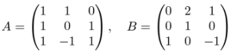
Let’s return to a concrete example of the nine numbers that specify a 3D linear transformation. Suppose a is a linear transformation, and we know a(e₁) = (1, 1, 1), a(e₂) = (1, 0, −1), and a(e₃) = (0, 1, 1). These three vectors having nine components in total contain all of the information required to specify the linear transformation a.

Because we reuse this concept over and over, it warrants a special notation. We’ll adopt a new notation, called matrix notation , to work with these nine numbers as a representation of a.

5.1.1 Writing vectors and linear transformations as matrices

Matrices are rectangular grids of numbers, and their shapes tell us how to interpret them. For instance, we can interpret a matrix that is a single column of numbers as a vector with its entries being the coordinates, ordered top to bottom. In this form, the vectors are called column vectors . For example, the standard basis for three dimensions can be written as three column vectors like this:

For our purposes, this notation means the same thing as e₁ = (1, 0, 0), e₂ = (0, 1, 0), and e₃ = (0, 0, 1). We can indicate how a transforms standard basis vectors with this notation as well:

The matrix representing the linear transformation a is the 3-by−3 grid consisting of these vectors squashed together side by side:

In 2D, a column vector consists of two entries, so 2 transformed vectors contain a total of 4 entries. We can look at the linear transformation D that scales input vectors by a multiple of 2. First, we write how it works on basis vectors:

Then the matrix for D is obtained by putting these columns next to each other:

Matrices can come in other shapes and sizes, but we’ll focus on these two shapes for now: the single column matrices representing vectors and the square matrices representing linear transformations.

Remember, there are no new concepts here, only a new way of writing the core idea from section 4.2: a linear transformation is defined by its results acting on the standard basis vectors. The way to get a matrix from a linear transformation is to find the vectors it produces from all of the standard basis vectors and combine the results side by side. Now, we’ll look at the opposite problem: how to evaluate a linear transformation given its matrix.

5.1.2 Multiplying a matrix with a vector

If a linear transformation B is represented as a matrix, and a vector v is also represented as a matrix (a column vector), we have all of the numbers required to evaluate B(v). For instance, if B and v are given by

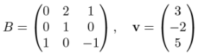
then the vectors B(e₁), B(e₂), and B(e₃) can be read off of B as the columns of its matrix. From that point, we use the same procedure as before. Because v = 3e₁ − 2e₂ + 5e₃, it follows that B(v) = 3 B(e₁) − 2 B(e₂) + 5 B(e₃). Expanding this, we get

and the result is the vector (1, −2, −2). Treating a square matrix as a function that operates on a column vector is a special case of an operation called matrix multiplication . Again, this has an impact on our notation and terminology, but we are simply doing the same thing: applying a linear transformation to a vector. Written as a matrix multiplication, it looks like this:

As opposed to multiplying numbers, the order matters when you multiply matrices by vectors. In this case, B v is a valid product but v B is not. Shortly, we’ll see how to multiply matrices of various shapes and a general rule for the order in which matrices can be multiplied. For now, take my word for it and think of this multiplication as valid because it means applying a 3D linear operator to a 3D vector.

We can write Python code that multiplies a matrix by a vector. Let’s say we encode the matrix B as a tuple-of-tuples and the vector v as a tuple as usual:

 B = (
    (0,2,1),
    (0,1,0),
    (1,0,−1)
)

v = (3,−2,5)

This is a bit different from how we originally thought about the matrix B. We originally created it by combining three columns, but here B is created as a sequence of rows. The advantage of defining a matrix in Python as a tuple of rows is that the numbers are laid out in the same order as we would write them on paper. We can, however, get the columns any time we want by using Python’s zip function (covered in appendix B):

>>> list(zip(*B))
[(0, 0, 1), (2, 1, 0), (1, 0, −1)]

The first entry of this list is (0, 0, 1), which is the first column of B, and so on. What we want is the linear combination of these vectors, where the scalars are the coordinates of v. To get this, we can use the linear_combination function from the exercise in section 4.2.5. The first argument to linear_combination should be v, which serves as the list of scalars, and the subsequent arguments should be the columns of B. Here’s the complete function:

def multiply_matrix_vector(matrix, vector):
    return linear_combination(vector, *zip(*matrix))

It confirms the calculation we did by hand with B and v :

>>> multiply_matrix_vector(B,v)
(1, −2, −2)

There are two other mnemonic recipes for multiplying a matrix by a vector, both of which give the same results. To see these, let’s write a prototypical matrix multiplication:

The result of this calculation is the linear combination of the columns of the matrix with the coordinates x, y, and z as the scalars:

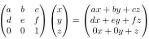
This is an explicit formula for the product of a 3-by−3 matrix with a 3D vector. You can write a similar one for a 2D vector:

The first mnemonic is that each coordinate of the output vector is a function of all the coordinates of the input vector. For instance, the first coordinate of the 3D output is a function f(x, y, z) = ax + by + cz. Moreover, this is a linear function (in the sense that you used the word in high school algebra); it is a sum of a number times each variable. We originally introduced the term “linear transformation” because linear transformations preserve lines. Another reason to use that term: a linear transformation is a collection of linear functions on the input coordinates that give the respective output coordinates.

The second mnemonic presents the same formula differently: the coordinates of the output vector are dot products of the rows of the matrix with the target vector. For instance, the first row of the 3-by−3 matrix is (a, b, c) and the multiplied vector is (x, y, z), so the first coordinate of the output is (a, b, c) · (x, y, z) = ax + by + cz. We can combine our two notations to state this fact in a formula:

If your eyes are starting to glaze over from looking at so many letters and numbers in arrays, don’t worry. The notation can be overwhelming at first, and it takes some time to connect it to your intuition. There are more examples of matrices in this chapter, and the next chapter provides more review and practice as well.

5.1.3 Composing linear transformations by matrix multiplication

Some of the examples of linear transformations we’ve seen so far are rotations, reflections, rescalings, and other geometric transformations. What’s more, any number of linear transformations chained together give us a new linear transformation. In math terminology, the composition of any number of linear transformations is also a linear transformation.

Because any linear transformation can be represented by a matrix, any two composed linear transformations can be as well. In fact, if you want to compose linear transformations to build new ones, matrices are the best tools for the job.

NOTE Let me take off my mathematician hat and put on my programmer hat for a moment. Suppose you want to compute the result of, say, 1,000 composed linear transformations operating on a vector. This can come up if you are animating an object by applying additional, small transformations within every frame of the animation. In Python, it would be computationally expensive to apply 1,000 sequential functions because there is computational overhead for every function call. However, if you were to find a matrix representing the composition of 1,000 linear transformations, you would boil the whole process down to a handful of numbers and a handful of computations.

Let’s look at a composition of two linear transformations: a(B(v)), where the matrix representations of a and B are known to be the following:

Here’s how the composition works step by step. First, the transformation B is applied to v, yielding a new vector B(v), or B v if we’re writing it as a multiplication. Second, this vector becomes the input to the transformation a, yielding a final 3D vector as a result: a(B v). Once again, we’ll drop the parentheses and write a(B v) as the product AB v. Writing this product out for v = (x, y, z) gives us a formula that looks like this:

If we work right to left, we know how to evaluate this. Now I’m going to claim that we can work left to right as well and get the same result. Specifically, we can ascribe meaning to the product matrix AB on its own; it will be a new matrix (to be discovered) representing the composition of the linear transformations a and B :

Now, what should the entries of this new matrix be? Its purpose is to represent the composition of the transformations a and B, which give us a new linear transformation, AB. As we saw, the columns of a matrix are the results of applying its transformation to standard basis vectors. The columns of the matrix AB are the result of applying the transformation AB to each of e₁, e₂, and e₃.

The columns of AB are, therefore, AB(e₁), AB(e₂) and AB(e₃). Let’s look at the first column, for instance, which should be AB(e₁) or a applied to the vector B(e₁). In other words, to get the first column of AB, we multiply a matrix by a vector, an operation that we already practiced:

Similarly, we find that AB(e₂) = (3, 2, 1) and AB(e₃) = (1, 0, 0), which are the second and third columns of AB :

That’s how we do matrix multiplication. You can see there’s nothing to it besides carefully composing linear operators. Similarly, you can use mnemonics instead of reasoning through this process each time. Because multiplying a 3-by−3 matrix by a column vector is the same as doing three dot products, multiplying two 3-by−3 matrices together is the same as doing nine dot products−all possible dot products of rows of the first matrix with columns of the second as shown in figure 5.2.

Figure 5.2 Each entry of a product matrix is a dot product of a row of the first matrix with a column of the second matrix.

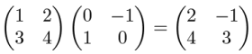
Everything we’ve said about 3-by−3 matrix multiplication applies to 2-by−2 matrices as well. For instance, to find the product of these 2-by−2 matrices

we can take the dot products of the rows of the first with the columns of the second. The dot product of the first row of the first matrix with the first column of the second matrix is (1, 2) · (0, 1) = 2. This tells us that the entry in the first row and first column of the result matrix is 2:

Repeating this procedure, we can find all the entries of the product matrix:

You can do some matrix multiplication as an exercise to get the hang of it, but you’ll quickly prefer that your computer does the work for you. Let’s implement matrix multiplication in Python to make this possible.

5.1.4 Implementing matrix multiplication

There are a few ways we could write our matrix multiplication function, but I prefer using the dot product trick. Because the result of matrix multiplication should be a tuple of tuples, we can write it as a nested comprehension. It takes in two nested tuples as well, called a and b, representing our input matrices a and B. The input matrix a is already a tuple of rows of the first matrix, and we can pair these up with zip(*b), which is a tuple of columns of the second matrix. Finally, for each pair, we should take the dot product and yield it in the inner comprehension. Here’s the implementation:

from vectors import *

def matrix_multiply(a,b):
    return tuple(
        tuple(dot(row,col) for col in zip(*b))
        for row in a
    )

The outer comprehension builds the rows of the result, and the inner one builds the entries of each row. Because the output rows are formed by the various dot products with rows of a , the outer comprehension iterates over a.

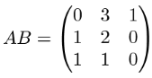
Our matrix_multiply function doesn’t have any hard-coded dimensions. That means we can use it to do the matrix multiplications from the preceding 2D and 3D examples:

>>> xa = ((1,1,0),(1,0,1),(1,−1,1))
>>> b = ((0,2,1),(0,1,0),(1,0,−1))
>>> matrix_multiply(a,b)
((0, 3, 1), (1, 2, 0), (1, 1, 0))
>>> xc = ((1,2),(3,4))
>>> d = ((0,−1),(1,0))
>>> matrix_multiply(c,d)
((2, −1), (4, −3))

Equipped with the computational tool of matrix multiplication, we can now do some easy manipulations of our 3D graphics.

5.1.5 3D animation with matrix transformations

To animate a 3D model, we redraw a transformed version of the original model in each frame. To make the model appear to move or change over time, we need to use different transformations as time progresses. If these transformations are linear transformations specified by matrices, we need a new matrix for every new frame of the animation.

Because PyGame’s built-in clock keeps track of time (in milliseconds), one thing we can do is to generate matrices whose entries depend on time. In other words, instead of thinking of every entry of a matrix as a number, we can think of it as a function that takes the current time, t, and returns a number (figure 5.3).

Figure 5.3 Thinking of matrix entries as functions of time allows the overall matrix to change as time passes.

For instance, we could use these nine expressions:

As we covered in chapter 2, cosine and sine are both functions that take a number and return another number as a result. The other five entries happen to not change over time, but if you crave consistency, you can think of these as constant functions (as in f(t) = 1 in the center entry). Given any value of t, this matrix represents the same linear transformation as rotate_y_by(t). Time moves forward and the value of t increases, so if we apply this matrix transformation to each frame, we’ll get a bigger rotation each time.

Let’s give our draw_model function (covered in appendix C and used extensively in chapter 4) a get_matrix keyword argument, where the value passed to get_matrix is a function that takes time in milliseconds and returns the transformation matrix that should be applied at that time. In the source code file, animate_teapot.py, I call it like this to animate the rotating teapot from chapter 4:

from teapot import load_triangles
from draw_model import draw_model
from math import sin,cos
 
def get_rotation_matrix(t):                   ❶
    seconds = t/1000                          ❷
    return (
        (cos(seconds),0,−sin(seconds)),
        (0,1,0),
        (sin(seconds),0,cos(seconds))
    )
draw_model(load_triangles(), 
           get_matrix=get_rotation_matrix)    ❸

❶ Generates a new transformation matrix for any numeric input representing time

❷ Converts the time to seconds so the transformation doesn’t happen too quickly

❸ Passes the function as a keyword argument to draw_model

Now, draw_model is passed the data required to transform the underlying teapot model over time, but we need to use it in the function’s body. Before iterating over the teapot faces, we execute the appropriate matrix transformation:

def draw_model(faces, color_map=blues, light=(1,2,3),
               camera=Camera("default_camera",[]),
               glRotatefArgs=None,
               get_matrix=None):
        #...                                                ❶
        def do_matrix_transform(v):                         ❷
            if get_matrix:                                  ❸
               m = get_matrix(pygame.time.get_ticks())
               return multiply_matrix_vector(m, v)
            else:
               return v                                      ❹
        transformed_faces = polygon_map(do_matrix_transform, 
                                        faces)              ❺
        for face in transformed_faces:
        #...                                                ❻

❶ Most of the function body is unchanged, so we don’t print it here.

❷ Creates a new function inside the main while loop that applies the matrix for this frame

❸ Uses the elapsed milliseconds given by pygame.time.get_ticks() as well as the provided get_matrix function to compute a matrix for this frame

❹ If no get_matrix is specified, doesn’t carry out any transformation and returns the vector unchanged

❺ Applies the function to every polygon using polygon_map

❻ The rest of the draw_model is the same as described in appendix C.

With these changes, you can run the code and see the teapot rotate (figure 5.4).

Figure 5.4 The teapot is transformed by a new matrix in every frame, depending on the elapsed time when the frame is drawn.

Hopefully, I’ve convinced you with the preceding examples that matrices are entirely interchangeable with linear transformations. We’ve managed to transform and animate the teapot the same way, using only nine numbers to specify each transformation. You can practice your matrix skills some more in the following exercises and then I’ll show you there’s even more to learn from the matrix_multiply function we’ve already implemented.

5.1.6 Exercises

def infer_matrix(n, transformation):
    def standard_basis_vector(i):
        return tuple(1 if i==j else 0 for j in range(1,n+1))         ❶
    standard_basis = [standard_basis_vector(i) for i in range(1,n+1)]❷
    cols = [transformation(v) for v  in standard_basis]               ❸
    return tuple(zip(*cols))                                         ❹

>>> from transforms import rotate_z_by
>>> from math import pi
>>> infer_matrix(3,rotate_z_by(pi/2))
((6.123233995736766e−17, −1.0, 0.0), (1.0, 1.2246467991473532e−16, 0.0), (0, 0, 1))

from random import randint
def random_matrix(rows,cols,min=−2,max=2):
    return tuple(
        tuple(
        randint(min,max) for j in range(0,cols))
        for i in range(0,rows)
    )

>>> random_matrix(3,3,0,10)
((3, 4, 9), (7, 10, 2), (0, 7, 4))

def transform(v):
    m = ((2,1,1),(1,2,1),(1,1,2))
    return multiply_matrix_vector(m,v)
draw_model(polygon_map(transform, load_triangles()))

def multiply_matrix_vector(matrix,vector):
    return tuple(
        sum(vector_entry * matrix_entry
            for vector_entry, matrix_entry in zip(row,vector))
        for row in matrix
    )

def multiply_matrix_vector(matrix,vector):
    return tuple(
        dot(row,vector)
        for row in matrix
    )

from transforms import compose

a = ((1,1,0),(1,0,1),(1,−1,1))
b = ((0,2,1),(0,1,0),(1,0,−1))

def transform_a(v):
    return multiply_matrix_vector(a,v)

def transform_b(v):
    return multiply_matrix_vector(b,v)

compose_a_b = compose(transform_a, transform_b)

>>> infer_matrix(3, compose_a_b)
((0, 3, 1), (1, 2, 0), (1, 1, 0))
>>> matrix_multiply(a,b)
((0, 3, 1), (1, 2, 0), (1, 1, 0))

def matrix_power(power,matrix):
    result = matrix
    for _ in range(1,power):
        result = matrix_multiply(result,matrix)
    return result

5.2 Interpreting matrices of different shapes

The matrix_multiply function doesn’t hard-code the size of the input matrices, so we can use it to multiply either 2-by−2 or 3-by−3 matrices together. As it turns out, it can also handle matrices of other sizes as well. For instance, it can handle these two 5-by−5 matrices:

>>> xa = ((−1, 0, −1, −2, −2), (0, 0, 2, −2, 1), (−2, −1, −2, 0, 1), (0, 2, −2,
−1, 0), (1, 1, −1, −1, 0))
>>> b = ((−1, 0, −1, −2, −2), (0, 0, 2, −2, 1), (−2, −1, −2, 0, 1), (0, 2, −2,
−1, 0), (1, 1, −1, −1, 0))
>>> matrix_multiply(a,b)
((−10, −1, 2, −7, 4), (−2, 5, 5, 4, −6), (−1, 1, −4, 2, −2), (−4, −5, −5, -9,
4), (−1, −2, −2, −6, 4))

There’s no reason we shouldn’t take this result seriously−our functions for vector addition, scalar multiplication, dot products, and, therefore, matrix multiplication don’t depend on the dimension of the vectors we use. Even though we can’t picture a 5D vector, we can do all the same algebra on five tuples of numbers that we did on pairs and triples of numbers in 2D and 3D, respectively. In this 5D product, the entries of the resulting matrix are still dot products of rows of the first matrix with columns of the second (figure 5.5):

Figure 5.5 The dot product of a row of the first matrix with a column of the second matrix produces one entry of the matrix product.

You can’t visualize it in the same way, but you can show algebraically that a 5-by−5 matrix specifies a linear transformation of 5D vectors. We spend time talking about what kind of objects live in four, five, or more dimensions in the next chapter.

5.2.1 Column vectors as matrices

Let’s return to the example of multiplying a matrix by a column vector. I already showed you how to do a multiplication like this, but we treated it as its own case with the multiply_matrix_vector function. It turns out matrix_multiply is capable of doing these products as well, but we have to write the column vector as a matrix. As an example, let’s pass the following square matrix and single-column matrix to our matrix_multiply function:

I claimed before that you can think of a vector and a single-column matrix interchangeably, so we might encode d as a vector (1,1,1). But this time, let’s force ourselves to think of it as a matrix, having three rows with one entry each. Note that we have to write (1,) instead of (1) to make Python think of it as a 1-tuple instead of as a number.

>>> xc = ((−1, −1, 0), (−2, 1, 2), (1, 0, −1))
>>> d = ((1,),(1,),(1,))
>>> matrix_multiply(c,d)
((−2,), (1,), (0,))

The result has three rows with one entry each, so it is a single-column matrix as well. Here’s what this product looks like in matrix notation:

Our multiply_matrix_vector function can evaluate the same product but in a different format:

>>> multiply_matrix_vector(c,(1,1,1))
(−2, 1, 0)

This demonstrates that multiplying a matrix and a column vector is a special case of matrix multiplication. We don’t need a separate function multiply_matrix _vector after all. We can further see that the entries of the output are dot products of the rows of the first matrix with the single column of the second (figure 5.6).

Figure 5.6 An entry of the resulting vector computed as a dot product

On paper, you’ll see vectors represented interchangeably as tuples (with commas) or as column vectors. But for the Python functions we’ve written, the distinction is critical. The tuple (−2, 1, 0) can’t be used interchangeably with the tuple-of-tuples ((−2,), (1,), (0,)). Yet another way of writing the same vector would be as a row vector , or a matrix with one row. Here are the three notations for comparison:

Table 5.1 Comparison of mathematical notations for vectors with corresponding Python representations

If you’ve seen this comparison in math class, you may have thought it was a pedantic notational distinction. Once we represent these in Python, however, we see that they are really three distinct objects that need to be treated differently. While these all represent the same geometric data, which is a 3D arrow or point in space, only one of these, the column vector, can be multiplied by a 3-by−3 matrix. The row vector doesn’t work because, as shown in figure 5.7, we can’t take the dot product of a row of the first matrix with a column of the second.

Figure 5.7 Two matrices that cannot be multiplied together

For our definition of matrix multiplication to be consistent, we can only multiply a matrix on the left of a column vector. This prompts the general question posed by the next section.

5.2.2 What pairs of matrices can be multiplied?

We can make grids of numbers of any dimension. When can our matrix multiplication formula work, and what does it mean when it does?

The answer is that the number of columns of the first matrix has to match the number of rows of the second. This is clear when we do the matrix multiplication in terms of dot products. For instance, we can multiply any matrix with three columns by a second matrix with three rows. This means that rows of the first matrix and columns of the second each have three entries, so we can take their dot products. Figure 5.8 shows the dot product of the first row of the first matrix with the first column of the second matrix gives us an entry of the product matrix.

Figure 5.8 Finding the first entry of the product matrix

We can complete this matrix product by taking the remaining seven dot products. Figure 5.9 shows another entry, computed from a dot product.

Figure 5.9 Finding another entry of the product matrix

This constraint also makes sense in terms of our original definition of matrix multiplication: the columns of the output are each linear combinations of the columns of the first matrix with scalars given by a row of the second matrix (figure 5.10).

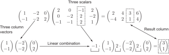
Figure 5.10 Each column of the result is a linear combination of the columns of the first matrix.

I was calling the previous square matrices 2-by−2 and 3-by−3 matrices. The last example (figure 5.10) was the product of a 2-by−3 and a 3-by−4 matrix. When we describe the dimensions of a matrix like this, we say the number of rows first and then the number of columns. For instance, a 3D column vector would be a 3-by−1 matrix.

Note Sometimes you’ll see matrix dimensions written with a multiplication sign as in a 3×3 matrix or a 3×1 matrix.

In this language, we can make a general statement about the shapes of matrices that can be multiplied: you can only multiply an n- by -m matrix by a p -by- q matrix if m = p. When that is true, the resulting matrix will be a n -by- q matrix. For instance, a 17×9 matrix cannot be multiplied by a 6×11 matrix. However, a 5×8 matrix can be multiplied by an 8×10 matrix. Figure 5.11 shows the result of the latter, which is a 5×10 matrix.

Figure 5.11 Each of the five rows of the first matrix can be paired with one of the ten columns of the second matrix to produce one of the 5 × 10 = 50 entries of the product matrix. I used stars instead of numbers to show you that any matrices of these sizes are compatible.

By contrast, you couldn’t multiply these matrices in the opposite order: a 10×8 matrix can’t be multiplied by a 5×8 matrix. Now it’s clear how to multiply bigger matrices, but what do the results mean? It turns out we can learn something from the result: all matrices represent vector functions, and all valid matrix products can be interpreted as composition of these functions. Let’s see how this works.

5.2.3 Viewing square and non-square matrices as vector functions

We can think of a 2×2 matrix as the data required to do a given linear transformation of a 2D vector. Pictured as a machine in figure 5.12, this transformation takes a 2D vector into its input slot and produces a 2D vector out of its output slot as a result.

Figure 5.12 Visualizing a matrix as a machine that takes vectors as inputs and produces vectors as outputs

Under the hood, our machine does this matrix multiplication:

It’s fair to think of matrices as machines that take vectors as inputs and produce vectors as outputs. Figure 5.13, however, shows a matrix can’t take just any vector as input; it is a 2×2 matrix so it does a linear transformation of 2D vectors. Correspondingly, this matrix can only be multiplied by a column vector with two entries. Let’s split up the machine’s input and output slots to suggest that these take and produce 2D vectors or pairs of numbers.

Figure 5.13 Refining our mental model by redrawing the machine’s input and output slots to indicate that its inputs and outputs are pairs of numbers

Likewise, a linear transformation machine (figure 5.14) powered by a 3×3 matrix can only take in 3D vectors and produce 3D vectors as a result.

Figure 5.14 A linear transformation machine powered by a 3×3 matrix takes in 3D vectors and outputs 3D vectors.

Now we can ask ourselves, what would a machine look like if it were powered by a non-square matrix? Perhaps the matrix would look something like this:

As a specific example, what kinds of vectors could this 2×3 matrix act on? If we’re going to multiply this matrix with a column vector, the column vector must have three entries to match the size of the rows of this matrix. Multiplying our 2×3 matrix by a 3×1 column vector gives us a 2×1 matrix as a result, or a 2D column vector. For example,

This tells us that this 2×3 matrix represents a function taking 3D vectors to 2D vectors. If we were to draw it as a machine, like in figure 5.15, it would accept 3D vectors in its input slot and produce 2D vectors from its output slot.

Figure 5.15 A machine that takes in 3D vectors and outputs 2D vectors, powered by a 2×3 matrix

In general, an m -by- n matrix defines a function taking n -dimensional vectors as inputs and returning m -dimensional vectors as outputs. Any such function is linear in the sense that it preserves vector sums and scalar multiples. It’s not a transformation because it doesn’t just modify input, it returns an entirely different kind of output: a vector living in a different number of dimensions. For this reason, we’ll use a more general terminology; we’ll call it a linear function or a linear map. Let’s consider an in-depth example of a familiar linear map from 3D to 2D.

5.2.4 Projection as a linear map from 3D to 2D

We already saw a vector function that accepts 3D vectors and produces 2D vectors: a projection of a 3D vector onto the x,y plane (section 3.5.2). This transformation (we can call it P) takes vectors of the form (x, y, z) and returns these with their z component deleted: (x, y). I’ll spend some time carefully showing why this is a linear map and how it preserves vector addition and scalar multiplication.

First of all, let’s write P as a matrix. To accept 3D vectors and return 2D vectors, it should be a 2×3 matrix. Let’s follow our trusty formula for finding a matrix by testing the action of P on standard basis vectors. Remember, in 3D the standard basis vectors are defined as e₁ = (1, 0, 0), e₂ = (0, 1, 0), and e₃ = (0, 0, 1), and when we apply the projection to these three vectors, we get (1, 0), (0, 1), and (0, 0), respectively. We can write these as column vectors

and then stick them together side by side to get a matrix:

To check this, let’s multiply it by a test vector (a, b, c). The dot product of (a, b, c) with (1, 0, 0) is a, so that’s the first entry of the result. The second entry is the dot product of (a, b, c) with (0, 1, 0), or b. You can picture this matrix as grabbing a and b from (a, b, c) and ignoring c(figure 5.16).

Figure 5.16 Only 1 · a contributes to the first entry of the product, and only 1 · b contributes to the second entry. The other entries are zeroed out (in gray in the figure).

This matrix does what we want; it deletes the third coordinate of a 3D vector, leaving us with only the first two coordinates. It’s good news that we can write this projection as a matrix, but let’s also give an algebraic proof that this is a linear map. To do this, we have to show that the two key conditions of linearity are satisfied.

Proving that projection preserves vector sums

If P is linear, any vector sum u + v = w should be respected by P. That is, P(u) + P(v) should equal P(w) as well. Let’s confirm this using these equations: u = (u₁, u₂, u₃) and v = (v₁, v₂, v₃). Then w = u + v so that

w = (u₁ + v₁, u₂ + v₂, u₃ + v₃)

Executing P on all of these vectors is simple because we only need to remove the third coordinate:

P(u) = (u₁, u₂)

P(v) = (v₁, v₂)

so

P(w) = (u₁ + v₁, u₂ + v₂)

Adding P(u) and P(v), we get (u₁ + v₁, u₂ + v₂), which is the same as P(w). For any three 3D vectors u + v = w, we, therefore, also have P(u) + P(v) = P(w). This validates our first condition.

Proving projection preserves scalar multiples

The second thing we need to show is that P preserves scalar multiples. Letting s stand for any real number and letting u = (u₁, u₂, u₃), we want to demonstrate that P(s u) is the same as sP(u).

Deleting the third coordinate and doing the scalar multiplication give the same result regardless of which order these operations are carried out. The result of s z is (su₁, su₂, su₃), so P(s u) = (su₁, su₂). The result of P(u) is (u₁, u₂), so sP(u) = (su₁, su₂). This validates the second condition and confirms that P satisfies the definition of linearity.

These kinds of proofs are usually easier to do than to follow, so I’ve given you another one as an exercise. In the exercise, you can check that a function from 2D to 3D, specified by a given matrix, is linear using the same approach.

More illustrative than an algebraic proof is an example. What does it look like when we project a 3D vector sum down to 2D? We can see it in three steps. First, we can draw a vector sum of two vectors u and v in 3D as shown in figure 5.17.

Figure 5.17 A vector sum of two arbitrary vectors z and v in 3D

Then, we can trace a line from each vector to the x,y plane to show where these vectors end up after projection (figure 5.18).

Figure 5.18 Visualizing where u, v, and z + v end up after projection to the x,y plane

Finally, we can look at these new vectors and see that they still constitute a vector sum (figure 5.19).

Figure 5.19 The projected vectors form a sum: P(v) + P(v) = P(u + v).

In other words, if three vectors u, v, and w form a vector sum u + v = w, then their “shadows” in the x,y plane also form a vector sum. Now that you’ve got some insight into linear transformation from 3D to 2D and a matrix that represents it, let’s return to our discussion of linear maps in general.

5.2.5 Composing linear maps

The beauty of matrices is that they store all of the data required to evaluate a linear function on a given vector. What’s more, the dimensions of a matrix tell us the dimensions of input vectors and output vectors for the underlying function. We captured that visually in figure 5.20 by drawing machines for matrices of varying dimensions, whose input and output slots have different shapes. Here are four examples we’ve seen, labeled with letters so we can refer back to them.

Figure 5.20 Four linear functions represented as machines with input and output slots. The shape of a slot tells us what dimension of vector it accepts or produces.

Drawn like this, it’s easy to pick out which pairs of linear function machines could be welded together to build a new one. For instance, the output slot of M has the same shape as the input slot of P, so we could make the composition P(M(v)) for a 3D vector v. The output of M is a 3D vector that can be passed right along into the input slot of P(figure 5.21).

Figure 5.21 The composition of P and M. A vector is passed into the input slot of M, the output M(v) passes invisibly through the plumbing and into P, and the output P(M(v)) emerges from the other end.

By contrast, figure 5.22 shows that we can’t compose N and M because N doesn’t have enough output slots to fill every input of M.

Figure 5.22 The composition of N and M is not possible because outputs of N are 2D vectors, while inputs to M are 3D vectors.

I’m making this idea visual now by talking about slots, but hidden underneath is the same reasoning we use to decide if two matrices can be multiplied together. The count of the columns of the first matrix has to match the count of rows of the second. When the dimensions match in this way, so do the slots, and we can compose the linear functions and multiply their matrices.

Thinking of P and M as matrices, the composition of P and M is written PM as a matrix product. (Remember, if PM acts on a vector v as PM v, M is applied first and then P.) When v = (1, 1, 1), the product PM v is a product of two matrices and a column vector, and it can be simplified into a single matrix times a column vector if we evaluate PM ( figure 5.23).

Figure 5.23 Applying M and then P is equivalent to applying the composition PM. We consolidate the composition into a single matrix by doing the matrix multiplication.

As a programmer, you’re used to thinking of functions in terms of the types of data they consume and produce. I’ve given you a lot of notation and terminology to digest thus far in this chapter, but as long as you grasp this core concept, you’ll get the hang of it eventually.

I strongly encourage you to work through the following exercises to make sure you understand the language of matrices. For the rest of this chapter and the next, there won’t be many big new concepts, only applications of what we’ve seen so far. These applications will give you even more practice with matrix and vector computations.

5.2.6 Exercises

>>> from vectors import dot
>>> dot((1,1),(1,1,1))
2

def transpose(matrix):
    return tuple(zip(*matrix))

>>> transpose(((1,),(2,),(3,)))
((1, 2, 3),)
>>> transpose(((1, 2, 3),))
((1,), (2,), (3,))

>>> def project_xy(v):
...     x,y,z = v
...     return (x,y)
...
>>> infer_matrix(3,project_xy)
((1, 0, 0), (0, 1, 0))

5.3 Translating vectors with matrices

One advantage of matrices is that computations look the same in any number of dimensions. We don’t need to worry about picturing the configurations of vectors in 2D or 3D; we can simply plug them into the formulas for matrix multiplication or use them as inputs to our Python matrix_multiply. This is especially useful when we want to do computations in more than three dimensions.

The human brain isn’t wired to picture vectors in four or five dimensions, let alone 100, but we already saw we can do computations with vectors in higher dimensions. In this section, we’ll cover a computation that requires doing computation in higher dimensions: translating vectors using a matrix.

5.3.1 Making plane translations linear

In the last chapter, we showed that translations are not linear transformations. When we move every point in the plane by a given vector, the origin moves and vector sums are not preserved. How can we hope to execute a 2D transformation with a matrix if it is not a linear transformation?

The trick is that we can think of our 2D points to translate as living in 3D. Let’s return to our dinosaur from chapter 2. The dinosaur was composed of 21 points, and we could connect these in order to create the outline of the figure:

from vector_drawing import *
 
dino_vectors = [(6,4), (3,1), (1,2), (−1,5), (−2,5), (−3,4), (−4,4),
    (−5,3), (−5,2), (−2,2), (−5,1), (−4,0), (−2,1), (−1,0), (0,−3),
    (−1,−4), (1,−4), (2,−3), (1,−2), (3,−1), (5,1)
]
 
draw(
    Points(*dino_vectors),
    Polygon(*dino_vectors)
)

The result is the familiar 2D dinosaur (figure 5.24).

Figure 5.24 The familiar 2D dinosaur from chapter 2

If we want to translate the dinosaur to the right by 3 units and up by 1 unit, we could simply add the vector (3, 1) to each of the dinosaur’s vertices. But this isn’t a linear map, so we can’t produce a 2×2 matrix that does this translation. If we think of the dinosaur as an inhabitant of 3D space instead of the 2D plane, it turns out we can formulate the translation as a matrix.

Bear with me for a moment while I show you the trick; I’ll explain how it works shortly. Let’s give every point of the dinosaur a z-coordinate of 1. Then we can draw it in 3D by connecting each of the points with segments and see that the resulting polygon lies on the plane where z = 1 (figure 5.25). I’ve created a helper function called polygon_segments_3d to get the segments of the dinosaur polygon in 3D.

from draw3d import *
def polygon_segments_3d(points,color='blue'):
    count = len(points)
    return [Segment3D(points[i], points[(i+1) % count],color=color) for i in range(0,count)]

dino_3d = [(x,y,1) for x,y in dino_vectors]

draw3d(
    Points3D(*dino_3d, color='blue'),
    *polygon_segments_3d(dino_3d)
)

Figure 5.25 The same dinosaur with each of its vertices given a z-coordinate of 1

Figure 5.26 shows a matrix that “skews” 3D space, so that the origin stays put, but the plane where z = 1 is translated as desired. Trust me for now! I’ve highlighted the numbers relating to the translation that you should pay attention to.

Figure 5.26 A magic matrix that moves the plane z = 1 by +3 in the x direction and by +1 in the y direction

We can apply this matrix to each vertex of the dinosaur and then voila! The dinosaur is translated by (3, 1) in its plane (figure 5.27).

Figure 5.27 Applying the matrix to every point keeps the dinosaur in the same plane, but translates it within the plane by (3, 1)..

Here’s the code:

magic_matrix = (
    (1,0,3),
    (0,1,1),
    (0,0,1))

translated = [multiply_matrix_vector(magic_matrix, v) for v  in dino_vectors_3d]

For clarity, we could then delete the z-coordinates again and show the translated dinosaur in the plane with the original one (figure 5.28).

Figure 5.28 Dropping the translated dinosaur back into 2D

You can reproduce the code and check the coordinates to see that the dinosaur was indeed translated by (3, 1) in the final picture. Now let me show you how the trick works.

5.3.2 Finding a 3D matrix for a 2D translation

The columns of our “magic” matrix, like the columns of any matrix, tell us where the standard basis vectors end up after being transformed. Calling this matrix T, the vectors e₁, e₂, and e₃ would be transformed into the vectors T e₁ = (1, 0, 0), T e₂ = (0, 1, 0), and T e₃ = (3, 1, 1). This means e₁ and e₂ are unaffected, and e₃ changes only its x − and y -components (figure 5.29).

Figure 5.29 This matrix doesn’t move e1 or e2, but it does move e3.

Any point in 3D and, therefore, any point on our dinosaur is built as a linear combination of e₁, e₂, and e₃. For instance, the tip of the dinosaur’s tail is at (6, 4, 1), which is 6e₁ + 4e₂ + e₃. Because T doesn’t move e₁ or e₂, only the effect on e₃ moves the point, T(e₃) = e₃ + (3, 1, 0), so that the point is translated by +3 in the x direction and +1 in the y direction. You can also see this algebraically. Any vector (x, y, 1) is translated by (3, 1, 0) by this matrix:

If you want to translate a collection of 2D vectors by some vector (a, b), the general steps are as follows:

1. Move the 2D vectors into the plane in 3D space, where z = 1 and each has a z-coordinate of 1.

2. Multiply the vectors by the matrix with your given choices of a and b plugged in:

   

3. Delete the z-coordinate of all of the vectors so you are left with 2D vectors as a result.

Now that we can do translations with matrices, we can creatively combine them with other linear transformations.

5.3.3 Combining translation with other linear transformations

In the previous matrix, the first two columns are exactly e₁ and e₂, meaning that only the change in e₃ moves a figure. We don’t want T(e₁) or T(e₂) to have any z-component because that would move the figure out of the plane z = 1. But we can modify or interchange the other components (figure 5.30).

Figure 5.30 Let’s see what happens when we move T(e1) and T(e2) in the x,y plane.

It turns out you can put any 2×2 matrix in the top left (as shown by figure 5.30) by doing the corresponding linear transformation in addition to the translation specified in the third column. For instance, this matrix

produces a 90° counterclockwise rotation. Inserting it in the translation matrix, we get a new matrix that rotates the x,y plane by 90° and then translates it by (3, 1) as shown in figure 5.31.

Figure 5.31 A matrix that rotates e1 and e3 by 90° and translates e3 by (3, 1). Any figure in the plane where z = 1 experiences both transformations.

To show this works, we can carry out this transformation on all of the 3D dinosaur vertices in Python. Figure 5.32 shows the output of the following code:

rotate_and_translate = ((0,−1,3),(1,0,1),(0,0,1))
rotated_translated_dino = [
    multiply_matrix_vector(rotate_and_translate, v) 
    for v  in dino_vectors_3d]

Figure 5.32 The original dinosaur (left) and a second dinosaur (right) that is both rotated and translated by a single matrix

Once you get the hang of doing 2D translations with a matrix, you can apply the same approach to doing a 3D translation. To do that, you’ll have to use a 4×4 matrix and enter the mysterious world of 4D.

5.3.4 Translating 3D objects in a 4D world

What is the fourth dimension? A 4D vector would be an arrow with some length, width, depth, and one other dimension. When we built 3D space from 2D space, we added a z-coordinate. That means that 3D vectors can live in the x,y plane, where z = 0, or they can live in any other parallel plane, where z takes a different value. Figure 5.33 shows some of these parallel planes.

Figure 5.33 Building 3D space out of a stack of parallel planes, each looking like the x,y plane but at different z-coordinates

We can think of four dimensions in analogy to this model: a collection of 3D spaces that are indexed by some fourth coordinate. One way to interpret the fourth coordinate is “time.” Each snapshot at a given time is a 3D space, but the collection of all of the snapshots is a fourth dimension called a spacetime . The origin of the spacetime is the origin of the space at the moment when time, t, is equal to 0 (figure 5.34).

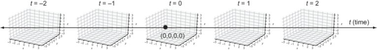
Figure 5.34 An illustration of 4D spacetime, similar to how a slice of 3D space at a given z value is a 2D plane and a slice of 4D spacetime at a given t value is a 3D space

This is the starting point for Einstein’s theory of relativity. (In fact, you are now qualified to go read about this theory because it is based on 4D spacetime and linear transformations given by 4×4 matrices.)

Vector math is indispensable in higher dimensions because we quickly run out of good analogies. For five, six, seven, or more dimensions, I have a hard time picturing them, but the coordinate math is no harder than in two or three dimensions. For our current purposes, it’s sufficient to think of a 4D vector as a four-tuple of numbers.

Let’s replicate the trick that worked for translating 2D vectors in 3D. If we start with a 3D vector like (x, y, z) and we want to translate it by a vector (a, b, c), we can attach a fourth coordinate of 1 to the target vector and use an analogous 4D matrix to do the translation. Doing the matrix multiplication confirms that we get the desired result (figure 5.35).

Figure 5.35 Giving the vector (x, y, z) a fourth coordinate of 1, we can translate the vector by (a, b, c) using this matrix.

This matrix increases the x-coordinate by a, the y-coordinate by b, and the z-coordinate by c, so it does the transformation required to translate by the vector (a, b, c). We can package in a Python function the work of adding a fourth coordinate, applying this 4×4 matrix, and then deleting the fourth coordinate:

def translate_3d(translation):
    def new_function(target):                    ❶
        a,b,c = translation
        x,y,z = target
        matrix = ((1,0,0,a),
            0,1,0,b),
            (0,0,1,c),
            (0,0,0,1))                           ❷
        vector = (x,y,z,1)
        x_out, y_out, z_out, _ =
          multiply_matrix_vector(matrix,vector)  ❸
        return (x_out,y_out,z_out)
    return new_function

❶ The translate_3d function takes a translation vector and returns a new function that applies that translation to a 3D vector.

❷ Builds the 4×4 matrix for the translation, and on the next line, turns (x, y, z) into a 4D vector with a fourth coordinate 1

❸ Does the 4D matrix transformation

Finally, drawing the teapot as well as the teapot translated by (2, 2, −3), we can see that the teapot moves appropriately. You can confirm this by running matrix_translate _teapot.py. You should see the same image as in figure 5.36.

Figure 5.36 The untranslated teapot (left) and a translated teapot (right). As expected, the translated teapot moves up and to the right, and away from our viewpoint.

With translation packaged as a matrix operation, we can now combine that operation with other 3D linear transformations and do them in one step. It turns out you can interpret the artificial fourth-coordinate in this setup as time, t.

The two images in figure 5.36 could be snapshots of a teapot at t = 0 and t = 1, which is moving in the direction (2, 2, −3) at a constant speed. If you’re looking for a fun challenge, you can replace the vector (x, y, z, 1) in this implementation with vectors of the form (x, y, z, t), where the coordinate t changes over time. With t = 0 and t = 1, the teapot should match the frames in figure 5.36, and at the time between the two, it should move smoothly between the two positions. If you can figure out how this works, you’ll catch up with Einstein!

So far, we’ve focused exclusively on vectors as points in space that we can render to a computer screen. This is clearly an important use case, but it only scratches the surface of what we can do with vectors and matrices. The study of how vectors and linear transformations work together in general is called linear algebra , and I’ll give you a broader picture of this subject in the next chapter, along with some fresh examples that are relevant to programmers.

5.3.5 Exercises

>>> from vectors import rotate2d
>>> from transforms import *
>>> from math import pi
>>> rotate_45_degrees = curry2(rotate2d)(pi/4)          ❶
>>> rotation_matrix = infer_matrix(2,rotate_45_degrees)
>>> rotation_matrix
((0.7071067811865476, -0.7071067811865475), (0.7071067811865475, 0.7071067811865476))

>>> from matrices import *
>>> scale_matrix = ((0.5,0),(0,0.5))
>>> rotate_and_scale = matrix_multiply(scale_matrix,rotation_matrix)
>>> rotate_and_scale
((0.3535533905932738, -0.35355339059327373), (0.35355339059327373, 0.3535533905932738))

>>> ((a,b),(c,d)) = rotate_and_scale
>>> final_matrix = ((a,b,2),(c,d,2),(0,0,1))
>>> final_matrix
((0.3535533905932738, -0.35355339059327373, 2), (0.35355339059327373, 0.3535533905932738, 2), (0, 0, 1))

def translate_4d(translation):
    def new_function(target):
        a,b,c,d = translation
        x,y,z,w = target
        matrix = (
            (1,0,0,0,a),
            (0,1,0,0,b),
            (0,0,1,0,c),
            (0,0,0,1,d),
            (0,0,0,0,1))
        vector = (x,y,z,w,1)
        x_out,y_out,z_out,w_out,_ = multiply_matrix_vector(matrix,vector)
        return (x_out,y_out,z_out,w_out)
    return new_function

>>> translate_4d((1,2,3,4))((10,20,30,40))
(11, 22, 33, 44)

In the previous chapters, we used visual examples in 2D and 3D to motivate vector and matrix arithmetic. As we’ve gone along, we’ve put more emphasis on computation. At the end of this chapter, we calculated vector transformations in higher dimensions where we didn’t have any physical insight. This is one of the benefits of linear algebra: it gives you the tools to solve geometric problems that are too complicated to picture. We’ll survey the broad range of this application in the next chapter.

Summary

• A linear transformation is defined by what it does to standard basis vectors. When you apply a linear transformation to the standard basis, the resulting vectors contain all the data required to do the transformation. This means that only nine numbers are required to specify a 3D linear transformation of any kind (the three coordinates of each of these three resulting vectors). For a 2D linear transformation, four numbers are required.

• In matrix notation, we represent a linear transformation by putting these numbers in a rectangular grid. By convention, you build a matrix by applying a transformation to the standard basis vectors and putting the resulting coordinate vectors side by side as columns.

• Using a matrix to evaluate the result of the linear transformation it represents on a given vector is called multiplying the matrix by the vector. When you do this multiplication, the vector is typically written as a column of its coordinates from top to bottom rather than as a tuple.

• Two square matrices can also be multiplied together. The resulting matrix represents the composition of the linear transformations of the original two matrices.

• To calculate the product of two matrices, you take the dot products of the rows of the first with the columns of the second. For instance, the dot product of row i of the first matrix and column j of the second matrix gives you the value in row i and column j of the product.

• As square matrices represent linear transformations, non-square matrices represent linear functions from vectors of one dimension to vectors of another dimension. That is, these functions send vector sums to vector sums and scalar multiples to scalar multiples.

• The dimension of a matrix tells you what kind of vectors its corresponding linear function accepts and returns. A matrix with m rows and n columns is called an m -by- n matrix (sometimes written m × n). It defines a linear function from n -dimensional space to m -dimensional space.

• Translation is not a linear function, but it can be made linear if you perform it in a higher dimension. This observation allows us to do translations (simultaneously with other linear transformations) by matrix multiplication.