This appendix covers the basic steps to get Python and related tools installed so you can run the code examples in this book. The main thing to install is Anaconda, which is a popular Python distribution for mathematical programming and data science. Specifically, Anaconda comes with an interpreter that runs Python code, as well as a number of the most popular math and data science libraries and a coding interface called Jupyter. The steps are mostly the same on any Linux, Mac, or Windows machine. I’m going to show you the steps on my Mac.
A.1 Checking for an existing Python installation
It’s possible you already have Python installed on your computer, even if you didn’t realize it. To check the existing installation, open a terminal window (or CMD or PowerShell on Windows) and type python. On a Mac straight from the factory, you should see a Python 2.7 terminal appear. You can press Ctrl-D to exit the terminal.

For the examples in this book, I use Python 3, which is becoming the new standard, and specifically, I use the Anaconda distribution. As a warning, if you have an existing Python installation, the following steps might be tricky. If any of the instructions below don’t work for you, my best advice is to search Google or StackOverflow with any error messages you see.
If you are a Python expert and don’t want to install or use Anaconda, you should be able to find and install the relevant libraries like NumPy, Matplotlib, and Jupyter using the pip package manager. For a beginner, I strongly recommend installing Anaconda as follows.
A.2 Downloading and installing Anaconda
Go to https://www.anaconda.com/distribution/ to download the Anaconda Python distribution. Click Download and choose the Python version beginning with 3 (figure A.1). At the time of writing, this was Python 3.7.

Figure A.1 At the time of writing, here’s what I see after clicking Download on the Anaconda website. To install Python, choose the Python 3.x download link.
Open the installer. It walks you through the installation process. The installer dialog box looks different depending on your operating system, but figure A.2 shows what it looks like on my Mac.

Figure A.2 The Anaconda installer as it appears on my Mac
I used the default installation location and didn’t add any optional features like the PyCharm IDE. Once the installation is complete, you should be able to open a fresh terminal. Type python to enter a Python 3 session with Anaconda (figure A.3).

Figure A.3 How the Python interactive session should look once you install Anaconda. Notice the Python 3.7.3 and the Anaconda, Inc. labels that appear.
If you don’t see a Python version starting with the number 3 and the word Anaconda, it probably means you’re stuck on the previous Python installation on your system. You need to edit your PATH environment variables so that your terminal knows which Python version you want when you type python in a terminal window. Hopefully, you won’t run into this problem, but if so, you can search online for a fix. You can also type python3 instead of python to explicitly use your Python 3 installation.
A.3 Using Python in interactive mode
Three angle brackets (>>>) in the terminal window prompt you to enter a line of Python code. When you type 2+2 and press Enter, you should see the Python interpreter’s evaluation of this statement, which is 4 (figure A.4).

Figure A.4 Entering a line of Python in the interactive session
Interactive mode is also referred to as a REPL, standing for read-evaluate-print loop. The Python session reads in a line of typed code, evaluates it, and prints the result, and this process is repeated as many times as you want in a loop. Pressing Ctrl-D signifies that you’re done entering code and sends you back to your terminal session.
Python interactive can usually identify if you enter a multi-line statement. For instance, def f(x): is the first line you enter when defining a new Python function called f. The Python interactive session shows you ... to indicate that it expects more input (figure A.5).
![]()
Figure A.5 The Python interpreter knows you’re not done with your multi-line statement.
You can indent to augment the function and then you need to press Enter twice to let Python know that you’ve finished the multi-line code input and to implement the function (figure A.6).
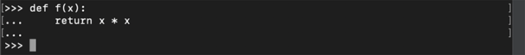
Figure A.6 Once you’ve completed your multi-line code, you need to press Enter twice to submit it.
The function f is now defined in your interactive session. On the next line, you can give Python input to evaluate (figure A.7).
![]()
Figure A.7 Evaluating the function defined previously
Beware that any code you write in an interactive session disappears when you exit the session. For that reason, if you’re writing a lot of code, it’s best to put it in a script file or in a Jupyter notebook. I’ll cover both of these methods next.
A.3.1 Creating and running a Python script file
You can create Python files with basically any text editor you like. As usual, it’s better to use a text editor designed for programming rather than a rich-text editor like Microsoft Word, which could insert invisible or unwanted characters for formatting. My preference is Visual Studio Code, and other popular choices are Atom, which is cross-platform, and Notepad++ for Windows. At your own risk, you can use a terminal-based text editor like Emacs or Vim. All of these tools are free and readily downloadable.
To create a Python script, simply create a new text file in your editor with a .py filename extension. Figure A.8 shows that I’ve created a file called first.py, which is in my ~/Documents directory. You can also see in figure A.8 that my text editor, Visual Studio Code, comes with syntax highlighting for Python. Keywords, functions, and literal values are colored to make it easy to read the code. Many editors (including Visual Studio Code) have optional extensions you can install to give you more helpful tools like checking for simple errors as you type, for instance.

Figure A.8 Some example Python code in a file. This code prints the squares of all digits from 0 to 9.
Figure A.8 shows a few lines of Python code typed into the first.py file. Because this is a math book, we can use an example that’s more “mathy” than Hello World. When we run the code, it prints the squares of all digits from 0 to 9.
Back in the terminal, go to the directory where your Python file lives. On my Mac, I go to the ~/Documents directory by typing cd ~/Documents. You can type ls first.py to confirm that you’re in the same directory as your Python script (figure A.9).

Figure A.9 The ls command shows you that the file first.py is in the directory.
To execute the script file, type python first.py into the terminal window. This invokes the Python interpreter and tells it to run the first.py file. The interpreter does what we hoped and prints some numbers (figure A.10).

Figure A.10 The result of running a simple Python script from the command line
When you’re solving more complicated problems, you might want to break your code up into separate files. Next, I’ll show you how to put the function f(x) in a different Python file that can be used by first.py. Let’s call this new file function.py and save it in the same directory as first.py, then cut and paste the code for f(x) into it (figure A.11).

Figure A.11 Putting the code to define the function f(x) in its own Python file
To let Python know that you’re going to combine multiple files in this directory, you need to add an empty text file called __init__.py in the directory. (That’s two underscores before and after the word init.)
Tip A quick way to create this empty file on a Mac or Linux machine is to type touch __init__.py.
To use the function f(x) from function.py in your script first.py, we need to let the Python interpreter know to retrieve it. To do that, we write from function import f as the first line in first.py (figure A.12).
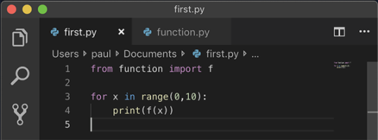
Figure A.12 Rewriting the file first.py to include the function f(x)
When you run the command python first.py again, you should get the same result as the previous time you ran it. This time, Python is getting the function f from function.py in the process.
An alternative to doing all of your work in text files and running them from the command line is to use Jupyter notebooks, which I’ll cover next. For this book, I did most of my examples in Jupyter notebooks, but I wrote any reusable code in separate Python files and imported those files.
A.3.2 Using Jupyter notebooks
A Jupyter Notebook is a graphical interface for coding in Python (and other languages as well). As with a Python interactive session, you type lines of code into a Jupyter notebook, and it prints the result. The difference is that Jupyter is a prettier interface than your terminal, and you can save your sessions to resume or re-run later.
Jupyter Notebook should automatically install with Anaconda. If you’re using a different Python distribution, you can install Jupyter with pip as well. See https://jupyter.org/install for documentation if you want to do a custom installation.
To open the Jupyter Notebook interface, type jupyter notebook or python -m notebook in a directory you want to work in. You should see a lot of text stream into the terminal, and your default web browser should open showing you the Jupyter Notebook interface.
Figure A.13 shows what I see in my terminal after typing python -m notebook. Again, your mileage may vary, depending on the Anaconda version you have.

Figure A.13 What the terminal looks like when you open a Jupyter notebook
Your default web browser should open, showing the Jupyter interface. Figure A.14 shows what I see when Jupyter opens in the Google Chrome browser.
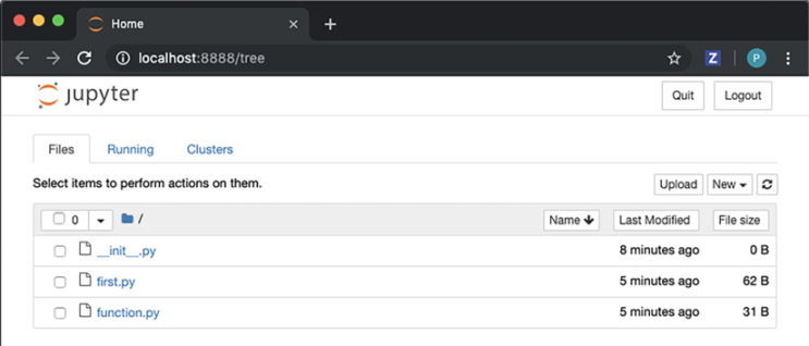
Figure A.14 When you start Jupyter, a browser tab automatically opens, looking something like this.
What’s going on here is that the terminal is running Python behind the scenes and also serving a local website at the address localhost:8888. From here on, you only have to think about what’s going on in the browser. The browser automatically sends the code you write to the Python process in the terminal via web requests. This Python background process is called a kernel in Jupyter terminology.
At the first screen that opens in the browser, you can see all of the files in the directory you’re working in. For example, I opened the notebook in my ~/Documents folder, so I can see the Python files we wrote in the last section. If you click one of the files, you’ll see you can view and edit it directly in the web browser. Figure A.15 shows what I see when I click first.py.
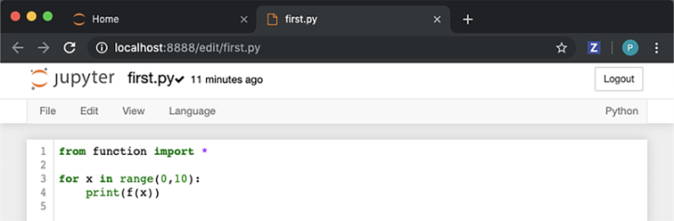
Figure A.15 Jupyter has a basic text editor for Python files. Here, I’ve opened the first.py file.
This isn’t a notebook yet. A notebook is a different kind of file than an ordinary Python file. To create a notebook, return to the main view by clicking the Jupyter logo in the top left corner, then go to the New dropdown menu on the right, and click Python 3 (figure A.16).

Figure A.16 Selecting the menu option to create a new Python 3 notebook
Once you’ve clicked Python 3, you’ll be taken to your new notebook. It should look like the one shown in figure A.17, with one blank input line ready to accept some Python code.

Figure A.17 A new, empty Jupyter notebook ready for coding
You can type a Python expression into the text box and then press Shift-Enter to evaluate it. In figure A.18, I typed 2+2 and then pressed Shift-Enter to see the output, 4.

Figure A.18 Evaluating 2 + 2 in a Jupyter notebook
As you can see, it works just like an interactive session except it looks nicer. Each input is shown in a box, and the corresponding output is shown below it.
If you just press Enter rather than Shift-Enter, you can add a new line inside your input box. In the interface, variables and functions defined in boxes above can be used by boxes below. Figure A.19 shows what our original example could look like in a Jupyter notebook.
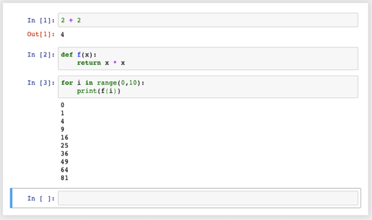
Figure A.19 Writing and evaluating several snippets of Python code in a Jupyter notebook. Notice the input boxes and the resulting output.
Strictly speaking, each box doesn’t depend on the boxes above it, but on the boxes you previously evaluated. For example, if I redefine the function f(x) in the next input box, and then rerun the previous box, I overwrite the previous output (figure A.20).

Figure A.20 If you redefine a symbol like f below the previous output and then rerun a box above, Python uses the new definition. Compare this figure with figure A.19 to see the new cell.
This can be confusing, but at least Jupyter renumbers the input boxes as you run them. For reproducibility, I suggest you define variables and functions above their first usage. You can confirm your code runs correctly from top to bottom by clicking the menu item Kernel > Restart & Run All (figure A.21). This wipes out all of your existing computations, but if you stay organized, you should get the same results back.

Figure A.21 Use the menu item Restart & Run All to clear the outputs and run all of your inputs from top to bottom.
Your notebook is automatically saved as you go. When you’re done coding, you can name the notebook by clicking Untitled at the top of the screen and entering a new name (figure A.22).

Figure A.22 Giving your notebook a name
Then you can click the Jupyter logo once again to return to the main menu, and you should see your new notebook saved as a file with the .ipynb extension (figure A.23). If you want to return to your notebook, you can click its name to open it.
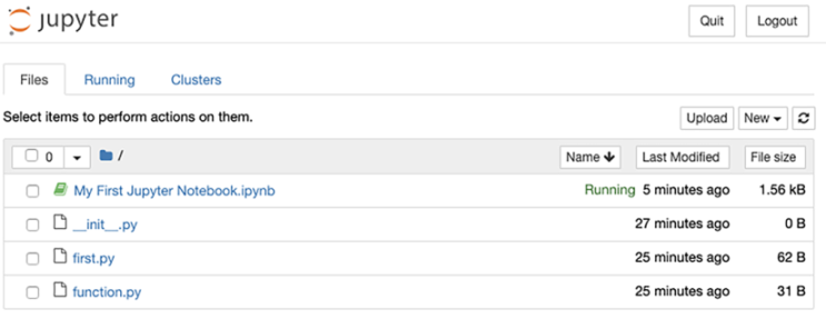
Figure A.23 Your new Jupyter notebook appears.
Tip To make sureall your files are saved, you should exit Jupyter by clicking Quit rather than just closing the browser tab or stopping the interactive process.
For more info on Jupyter notebooks, you can consult the extensive documentation at https://jupyter.org/. At this point, however, you know enough to download and play with the source code for this book, which is organized in a Jupyter notebook for almost all of the chapters.