This chapter covers

• Classifying images of handwritten digits as vector data
• Designing a type of neural network called a multilayer perceptron
• Evaluating a neural network as a vector transformation
• Fitting a neural network to data with a cost function and gradient descent
• Calculating partial derivatives for neural networks in backpropagation

In the final chapter of this book, we combine almost everything you’ve learned so far to introduce one of the most famous machine learning tools used today: artificial neural networks. Artificial neural networks, or neural networks for short, are mathematical functions whose structure is loosely based on the structure of the human brain. These are called artificial to distinguish from the “organic” neural networks that exist in the brain. This might sound like a lofty and complex goal, but it’s all based on a simple metaphor for how the brain works.

Before explaining the metaphor, I’ll preface this discussion by reminding you that I’m not a neurologist. The rough idea is that the brain is a big clump of interconnected cells called neurons and, when you think certain thoughts, what’s actually happening is electrical activity at specific neurons. You can see this electrical activity in the right kind of brain scan where various parts of the brain light up (figure 16.1).

Figure 16.1 Different kinds of brain activity cause different neurons to electrically activate, showing bright areas in a brain scan.

As opposed to the billions of neurons in the human brain, the neural networks we build in Python have only a few dozen neurons, and the degree to which a specific neuron is turned on is represented by a single number called its activation. When a neuron activates in the brain or in our artificial neural network, it can cause adjacent, connected neurons to turn on as well. This allows one idea to lead to another, which we can loosely see as creative thinking.

Mathematically, the activation of a neuron in our neural network is a function of the numerical activation values of neurons it is connected to. If a neuron connects to four others with the activation values a₁ , a₂ , a₃ , and a₄ , then its activation will be some mathematical function applied to those four values, say f(a₁ , a₂ , a₃ , a₄ ).

Figure 16.2 shows a schematic diagram with all of the neurons drawn as circles. I’ve shaded the neurons differently to indicate that they have different levels of activation, kind of like the brighter or darker areas of a brain scan.

Figure 16.2 Picturing neuron activation as a mathematical function, where a₁ , a₂ , a₃ , and a₄ are the activation values applied to the function f.

If each of a₁ , a₂ , a₃ , and a₄ depend on the activation of other neurons, the value of a could depend on even more numbers. With more neurons and more connections, you can build an arbitrarily complicated mathematical function, and the goal is to model arbitrarily complicated ideas.

The explanation I’ve just given you is a somewhat philosophical introduction to neural networks, and it’s definitely not enough for you to start coding. In this chapter, I show you, in detail, how to run with these ideas and build your own neural network. As in the last chapter, the problem we’ll solve with neural networks is classification. There are many steps in building a neural network and training it to perform well on classification, so before we dive in, I’ll lay out the plan.

16.1 Classifying data with neural networks

In this section, I focus on a classic application of neural networks: classifying images. Specifically, we’ll use low resolution images of handwritten digits (numbers from 0 to 9), and we want our neural network to identify which digit is shown in a given image. Figure 16.3 shows some example images for these digits.

Figure 16.3 Low resolution images of some handwritten digits

Figure 16.4 How our Python neural network function classifies images of digits.

If you identified the digits in figure 16.3 as 6, 0, 5, and 1, then congratulations! Your organic neural network (that is, your brain) is well trained. Our goal here is to build an artificial neural network that looks at such an image and classifies it as one of ten possible digits, perhaps as well as a human could.

In chapter 15, the classification problem amounted to looking at a 2D vector and classifying it in one of two classes. In this problem, we look at 8x8 pixel grayscale images, where each of the 64 pixels is described by one number that tells us its brightness. Just as we treated images as vectors in chapter 6, we’ll treat the 64-pixel brightness values as a 64-dimensional vector. We want to put each 64-dimensional vector in one of ten classes, indicating which digit it represents. Thus, our classification function will have more inputs and more outputs than the one in chapter 15.

Concretely, the neural network classification function we’ll build in Python will look like a function with 64 inputs and 10 outputs. In other words, it’s a (non-linear!) vector transformation from ℝ⁶⁴ to ℝ¹⁰ . The input numbers are the pixel darkness values, scaled from 0 to 1, and the ten output values represent how likely the image is to be any of the ten digits. The index of the largest output number is the answer. In the following case (shown by figure 16.4), an image of a 5 is passed in, and the neural network returns its largest value in the fifth slot, so it correctly identifies the digit in the image.

The neural network function in the middle of figure 16.4 is nothing more than a mathematical function. Its structure will be more complex than the ones we’ve seen so far, and in fact, the formula defining it is too long to write on paper. Evaluating a neural network is more like carrying out an algorithm. I’ll show you how to do this and implement it in Python.

Just as we tested many different logistic functions in the previous chapter, we could try many different neural networks and see which one has the best predictive accuracy. Once again, the systematic way to do this is a gradient descent. While a linear function is determined by the two constants a and b in the formula f(x) = ax + b, a neural network of a given shape can have thousands of constants determining how it behaves. That’s a lot of partial derivatives to take! Fortunately, due to the form of the functions connecting neurons in our neural network, there’s a shortcut algorithm for taking the gradient, which is called backpropagation.

It’s possible to derive the backpropagation algorithm from scratch and implement it using only the math we’ve covered so far, but unfortunately, that’s too big of a project to fit in this book. Instead, I’ll show you how to use a famous Python library called scikit-learn (“sci” pronounced as in “science”) to do the gradient descent for us, so it automatically trains the neural network to predict as well as possible for our data set. Finally, I’ll leave you with a teaser of the math behind backpropagation. I hope this will be just the starting point for your prolific career in machine learning.

16.2 Classifying images of handwritten digits

Before we start implementing our neural network, we need to prepare the data. The digit images I use are among the extensive, free test data that comes with the scikit-learn data. Once we download those, we need to convert them into 64-dimensional vectors with values scaled between zero and one. The data set also comes with the correct answers for each digit image, represented as Python integers from zero to nine.

Then we build two Python functions to practice the classification. The first is a fake digit identification function called random_classifier, which takes 64 numbers representing an image and (randomly) outputs 10 numbers representing the certainty that the image represents each digit from 0 to 9. The second is a function called test_digit_classify, which takes a classifier and automatically plugs in every image in the data set, returning a count of how many correct answers come out. Because our random_classifier produces random results, it should only guess the right answer 10% of the time. This sets the stage for improvement when we replace it with a real neural network.

16.2.1 Building the 64-dimensional image vectors

If you’re working with the Anacondas Python distribution as described in appendix A, you should already have the scikit-learn library available as sklearn. If not, you can install it with pip. To open sklearn and import the digits data set, you need the following code:

from sklearn import datasets
digits = datasets.load_digits()

Each entry of digits is a 2D NumPy array (a matrix), giving the pixel values of one image. For instance, digits.images[0] gives the pixel values of the first image in the data set, which is an 8-by-8 matrix of values:

>>> digits.images[0]
array([[ 0.,  0.,  5., 13.,  9.,  1.,  0.,  0.],
       [ 0.,  0., 13., 15., 10., 15.,  5.,  0.],
       [ 0.,  3., 15.,  2.,  0., 11.,  8.,  0.],
       [ 0.,  4., 12.,  0.,  0.,  8.,  8.,  0.],
       [ 0.,  5.,  8.,  0.,  0.,  9.,  8.,  0.],
       [ 0.,  4., 11.,  0.,  1., 12.,  7.,  0.],
       [ 0.,  2., 14.,  5., 10., 12.,  0.,  0.],
       [ 0.,  0.,  6., 13., 10.,  0.,  0.,  0.]])

Figure 16.5 The first image in sklearn’s digit data set, which looks like a zero

You can see that the range of grayscale values is limited. The matrix consists only of whole numbers from 0 to 15.

Matplotlib has a useful built-in function called imshow, which shows the entries of a matrix as an image. With the correct grayscale specification, the zeroes in the matrix appear as white and the bigger non-zero values appear as darker shades of gray. For instance, figure 16.5 shows the first image in the data set, which looks like a zero, resulting from imshow :

import matplotlib.pyplot as plt
plt.imshow(digits.images[0], cmap=plt.cm.gray_r)
 

To emphasize once more how we’re going to think of this image as a 64-dimensional vector, figure 16.6 shows a version of the image with each of the 64-pixel brightness values overlaid on the corresponding pixels.

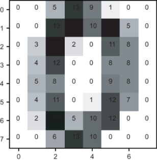
Figure 16.6 An image from the digit data set with brightness values overlaid on each pixel.

To turn this 8-by-8 matrix of numbers into a single 64-entry vector, we can use a built-in NumPy function called np .matrix.flatten. This function builds a vector starting with the first row of the matrix, followed by the second row, and so on, giving us a vector representation of an image similar to the one we used in chapter 6. Flattening the first image matrix indeed gives us a vector with 64 entries:

>>> import numpy as np
>>> np.matrix.flatten(digits.images[0])
array([ 0.,  0.,  5., 13.,  9.,  1.,  0.,  0.,  0.,  0., 13., 15., 10.,
       15.,  5.,  0.,  0.,  3., 15.,  2.,  0., 11.,  8.,  0.,  0.,  4.,
       12.,  0.,  0.,  8.,  8.,  0.,  0.,  5.,  8.,  0.,  0.,  9.,  8.,
        0.,  0.,  4., 11.,  0.,  1., 12.,  7.,  0.,  0.,  2., 14.,  5.,
       10., 12.,  0.,  0.,  0.,  0.,  6., 13., 10.,  0.,  0.,  0.])

To keep our analysis numerically tidy, we’ll once again scale our data so that the values are between 0 and 1. Because all the pixel values for every entry in this data set are between 0 and 15, we can scalar multiply these vectors by 1 / 15 to get scaled versions. NumPy overloads the * and / operators to automatically work as scalar multiplication (and division) of vectors, so we can simply type

np.matrix.flatten(digits.images[0]) / 15

and we’ll get a scaled result. Now we can build a sample digit classifier to plug these values into.

16.2.2 Building a random digit classifier

The input to the digit classifier is a 64-dimensional vector, like the ones we just constructed, and the output is a 10-dimensional vector with each entry value between 0 and 1. For our first example, the output vector entries can be randomly generated, but we interpret them as the classifier’s certainty that the image represents each of the ten digits.

Because we’re okay with random outputs for now, this is easy to implement; NumPy has a function, np.random.rand, that produces an array of random numbers between 0 and 1 of a specified size. For instance, np.random.rand(10) gives us a NumPy array of 10 random numbers between 0 and 1. Our random_classifier function takes an input vector, ignores it, and returns a random vector:

def random_classifier(input_vector):
    return np.random.rand(10)

To classify the first image in the data set, we can run the following:

>>> xv  = np.matrix.flatten(digits.images[0]) / 15.
>>> result = random_classifier(v)
>>> result
array([0.78426486, 0.42120868, 0.47890909, 0.53200335, 0.91508751,
       0.1227552 , 0.73501115, 0.71711834, 0.38744159, 0.73556909])

The largest entry of this output is about 0.915, occurring at index 4. Returning this vector, our classifier tells us that there’s some chance that the image represents any of the digits and that it is most likely a 4. To get the index of a maximum value programmatically, we can use the following Python code:

>>> list(result).index(max(result))
4

Here, max(result) finds the largest entry of the array, and list(result) treats the array as an ordinary Python list. Then we can use the built-in list index function to find the index of the maximum value. The return value of 4 is incorrect; we saw previously that the picture is a 0, and we can check the official result as well.

The correct digit for each image is stored at the corresponding index in the digits.target array. For the image digits.images[0], the correct value is digits.target[0], which is zero as we expected:

>>> digits.target[0]
0

Our random classifier predicted the image to be a 4 when in fact it was a 0. Because it is guessing at random, it should be wrong 90% of the time, and we can confirm this by testing it on a lot of test examples.

16.2.3 Measuring performance of the digit classifier

Now we’ll write the function test_digit_classify, which takes a classifier function and measures its performance on a large set of digit images. Any classifier function will have the same shape; it takes a 64-dimensional input vector and returns a 10-dimensional output vector. The test_digit_classify function goes through all of the test images and known correct answers and sees if the classifier produces the right answer:

def test_digit_classify(classifier,test_count=1000):
    correct = 0                                          ❶
    for img, target in zip(digits.images[:test_count], 
digits.target[:test_count]):                             ❷
        v  = np.matrix.flatten(img) / 15.                ❸
        output = classifier(v)                           ❹
        answer = list(output).index(max(output))         ❺
        if answer == target:
            correct += 1                                 ❻
    return (correct/test_count)                          ❼

❶ Starts the counter of correct classifications at 0

❷ Loops over pairs of images in the test set with corresponding targets, giving the correct answer for the digit

❸ Flattens the image matrix into a 64D vector and scales it appropriately

❹ Passes the image vector through the classifier to get a 10D result

❺ Finds the index of the largest entry in this result, which is the classifier’s best guess

❻ If this matches our answer, increments the counter

❼ Returns the number of correct classifications as a fraction of the total number of test data points

We expect our random classifier to get about 10% of the answers right. Because it acts randomly, it might do better on some trials than others, but because we’re testing on so many images, the result should be somewhere close to 10% every time. Let’s give it a try:

>>> test_digit_classify(random_classifier)
0.107

In this test, our random classifier did slightly better than expected at 10.7%. This isn’t too interesting on its own, but now we’ve got our data organized and a baseline example to beat so we can start building our neural network.

16.2.4 Exercises

array([5.00512567e-06, 3.94168539e-05, 5.57124430e-09, 9.31981207e-09,
       9.98060276e-01, 9.10328786e-07, 1.56262695e-03, 1.82976466e-04,
       1.48519455e-04, 2.54354113e-07])

def average_img(i):
    imgs = [img for img,target in zip(digits.images[1000:], digits.target[1000:]) if target==i]
    return sum(imgs) / len(imgs)

avg_digits = [np.matrix.flatten(average_img(i)) for i in range(10)]
def compare_to_avg(v):
    return [np.dot(v,avg_digits[i]) for i in range(10)]

>>> test_digit_classify(compare_to_avg)
0.853

16.3 Designing a neural network

In this section, I show you how to think of a neural network as a mathematical function and how you can expect it to behave, depending on its structure. That sets us up for the next section, where we implement our first neural network as a Python function in order to classify digit images.

For our image classification problem, our neural network has 64 input values and 10 output values, and requires hundreds of operations to evaluate. For that reason, in this section, I stick with a simpler neural network with three inputs and two outputs. This makes it possible to picture the whole network and walk through every step of its evaluation. Once we cover this, it will be easy to write the evaluation steps that work on a neural network of any size in general Python code.

16.3.1 Organizing neurons and connections

As I described in the beginning of this chapter, the model for a neural network is a collection of neurons, where a given neuron activates, depending on how much its connected neurons activate. Mathematically, turning on a neuron is a function of the activations of the connected neurons. Depending on how many neurons are used, which neurons are connected, and the functions that connect them, the behavior of a neural network can be different. In this chapter, we’ll restrict our attention to one of the simplest useful kinds of neural networks−a multilayer perceptron.

A multilayer perceptron, abbreviated MLP, consists of several columns of neurons called layers, arranged from left to right. Each neuron’s activation is a function of the activations in the previous layer, which is the layer immediately to the left. The leftmost layer depends on no other neurons, and its activation is based on training data. Figure 16.7 provides a schematic of a four-layer MLP.

Figure 16.7 A schematic of a multilayer perceptron (MLP), consisting of several layers of neurons

In figure 16.7, each circle is a neuron, and lines between the circles show connected neurons. Turning on a neuron depends only on the activations of neurons from the previous layer, and it influences the activations of every neuron in the next layer. I arbitrarily chose the number of neurons in each layer, and in this particular schematic, the layers consist of three, four, three, and two neurons, respectively.

Because there are 12 total neurons, there are 12 total activation values. Often there can be many more neurons (we’ll use 90 for digit classification), so we can’t give a letter variable name to every neuron. Instead, we represent all activations with the letter a and index them with superscripts and subscripts. The superscript indicates the layer, and the subscript indicates which neuron we’re talking about within the layer. For instance, a

is a number representing the activation of the second neuron in the second layer.

16.3.2 Data flow through a neural network

To evaluate a neural network as a mathematical function, there are three basic steps, which I describe in terms of the activation values. I’ll walk through them conceptually, and then I’ll show you the formulas. Remember, a neural network is just a function that takes an input vector and produces an output vector. The steps in between are just a recipe for getting to the output from the given input. Here’s the first step in the pipeline.

Step 1: Set the input layer activations to the entries of the input vector

The input layer is another word for the first or leftmost layer. The network in figure 16.7 has three neurons in the input layer, so this neural network can take 3D vectors as inputs. If our input vector is (0.3, 0.9, 0.5), then we can perform this first step by setting a₁⁰ = 0.3, a₂⁰ = 0.9, and a₃⁰ = 0.5. That fills in 3 of the 12 total neurons in the network (figure 16.8).

Figure 16.8 Setting the input layer activations to the entries of the input vector (left)

Each activation value in layer one is a function of the activations in layer zero. Now we have enough information to calculate them, so that’s step 2.

Step 2: Calculate each activation in the next layer as a function of all of the activations in the input layer

This step is the meat of the calculation, and I’ll return to it once I’ve gone through all of the steps conceptually. The important thing to know for now is that each activation in the next layer is usually given by a distinct function of the previous layer activations. Say we want to calculate a₀¹.This acti-vation is some function of a₁⁰ , a₂⁰ and a₃⁰ ,which we can simply write as a 1¹ = f(a₁⁰ , a₂⁰ , a₃⁰ )for now. Suppose, for instance, we calculate f(0.3, 0.9, 0.5) and the answer is 0.6. Then the value of a 1¹ becomes 0.6 in our calculation (figure 16.9).

Figure 16.9 Calculating an activation in layer one as some function of the activations in layer zero

When we calculate the next activation in layer one, a₂¹ ,it is also a function of the input activations a₁⁰ , a₂⁰ ,and a₃⁰ ,but in general, it is a different function, say a₂¹ = g(a₁⁰ , a₂⁰ , a₃⁰ ).The result still depends on the same inputs, but as a different function, it’s likely we’ll get a different result. Let’s say, g(0.3, 0.9, 0.5) = 0.1, then that’s our value for a₂¹ (figure 16.10).

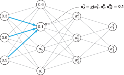
Figure 16.10 Calculating another activation in layer one with another function of the input layer activations

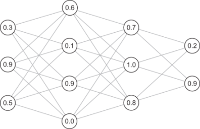
I used f and g because those are simple placeholder function names. There are two more distinct functions for a₃¹ and a₄¹ in terms of the input layer. I won’t keep naming these functions, because we’ll quickly run out of letters, but the important point is that each activation has a special function of the previous layer activations. Once we calculate all of the activations in layer one, we’ve 7 of the 12 total activations filled in. The numbers here are still made up, but the result might look something like that shown in figure 16.11.

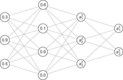
Figure 16.11 Two layers of activations for our multilayer perceptron (MLP) calculated.

From here on out, we repeat the process until we’ve calculated the activation of every neuron in the network, which is step 3.

Step 3: Repeat this process, calculating the activations of each subsequent layer based on the activations in the preceding layer

We start by calculating a₁² as a function of the layer one activations, a₁¹ , a₂¹ , a₃¹ ,and a₄¹ .Then we move on to a₂² and a₃² ,which are given by their own functions. Finally, we calculate a₁³ and a₂³ as their own functions of the layer two activations. At this point, we have an activation for every neuron in the network (figure 16.12).

Figure 16.12 An example of an MLP with all activations calculated

At this point, our calculation is done. We have activations calculated for the middle layers, called hidden layers, and the final layer, called the output layer. All we need to do now is to read off the activations of the output layer to get our result and that’s step 4.

Step 4: Return a vector whose entries are the activations of the output layer

In this case, the vector is (0.2, 0.9), so evaluating our neural network as a function of the input vector (0.3, 0.9, 0.5) produces the output vector (0.2, 0.9).

That’s all there is to it! The only thing I didn’t cover is how to calculate individual activations, and these are what make the neural network distinct. Every neuron, except for those in the input layer, has its own function, and the parameters defining those functions are the numbers we’ll tweak to make the neural network do what we want.

16.3.3 Calculating activations

The good news is that we’ll use a familiar form of function to calculate the activations in one layer as a function of those in the previous layer: logistic functions. The tricky part is that our neural network has 9 neurons outside the input layer, so there are 9 distinct functions to keep track of. What’s more, there are several constants to determine the behavior of each logistic function. Most of the work will be keeping track of all of these constants.

To focus on a specific example, we noted that in our sample MLP, we have the activation depend on the three input layer activations: a₁⁰ , a₂⁰ , and a₃⁰ .The function giving a₁¹ is a linear function of these inputs (including a constant) passed into a sigmoid function. There are four free parameters here, which I name a, B, C, and D for the moment (figure 16.13).

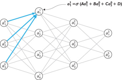
Figure 16.13 The general form of the function to calculate a11as a function of the input layer activations

We need to tune the variables a, B, C, and D to make a₁¹ respond appropriately to inputs. In chapter 15, we thought of logistic functions as taking in several numbers and making a yes-or-no decision about them, reporting the answer as a certainty of “yes” from zero to one. In that sense, you can think of the neurons in the middle of the network as breaking the overall classification problem into smaller yes-or-no classifications.

For every connection in the network, there is a constant telling us how strongly the input neuron activation affects the output neuron activation. In this case, the constant a tells us how strongly a₁⁰ affects a₁¹ ,while B and C tell us how strongly a₂⁰ and a₃⁰ affect a₁¹ ,respectively. These constants are called weights for the neural network, and there is one weight for every line segment in the neural network general diagram used throughout this chapter.

The constant D doesn’t affect the connection, but instead, independently increases or decreases the value of a₁¹ ,which is not dependent on an input activation. This is appropriately named the bias for the neuron because it measures the inclination to make a decision without any input. The word bias sometimes comes with a negative connotation, but it’s an important part of any decision-making process; it helps avoid outlier decisions unless there is strong evidence.

As messy as it might look, we need to index these weights and biases rather than giving them names like a, B, C, and D. We’ll write the weights in the form w_ij^l , where l is the layer on the right of the connection, i is the index of the previous neuron in layer l − 1, and j is the index of the target neuron in layer l. For instance, the weight a, which impacts the first neuron of layer one based on the value of the first neuron of layer zero is denoted by w₁₁¹ .The weight connecting the second neuron of layer three to the first neuron of the previous layer is w₂₁³ (figure 16.14).

Figure 16.14 Showing the connections corresponding to weights w₁₁¹ and w₃₂¹

The biases correspond to neurons, not pairs of neurons, so there is one bias for each neuron: b_j^l for the bias of the j th neuron in the i^th layer. In terms of these naming conventions, we could write the formula for a₁¹ as

a₁¹ = σ(w₁₁¹ a₁⁰ + w₁₂² a₂⁰ + w₁₃³ a₃⁰ + b₁¹)

or the formula for a₃² as

a₃² = σ(w₃₁² a₁¹ + w₃₂² a₂¹ + w₃₃² a₃¹ + w₃₄² a₄¹ + b₃²)

As you can see, computing activations to evaluate an MLP is not difficult, but the number of variables can make it a tedious and error-prone process. Fortunately, we can simplify the process and make it easier to implement using the notation of matrices we covered in chapter 5.

16.3.4 Calculating activations in matrix notation

As nasty as it could be, let’s do a concrete example and write the formula for the activations of a whole layer of the network, and then we’ll see how to simplify it in matrix notation and write a reusable formula. Let’s take layer two. The formulas for the three activations are as follows:

a₁² = σ(w₁₁² a₁¹ + w₁₂² a₂¹ + w₁₃² a₃¹ + w₁₄² a₄¹ + b₁²)

a₂² = σ(w₂₁² a₁¹ + w₂₂² a₂¹ + w₂₃² a₃¹ + w₂₄² a₄¹ + b₂²)

a₃² = σ(w₃₁² a₁¹ + w₃₂² a₂¹ + w₃₃² a₃¹ + w₃₄² a₄¹ + b₃²)

It turns out to be useful to name the quantities inside the sigmoid function. Let’s denote the three quantities z₁², z₂², and z₃²,so that by definition

a₁² = σ(z₁²)

a₂² = σ(z₂²)

and

a₃² = σ(z₃²)

The formulas for these z values are nicer because they are all linear combinations of the previous layer activations, plus a constant. That means we can write them in matrix vector notation. Starting with

z₁² = w₁₁² a₁¹ + w₁₂² a₂¹ + w₁₃² a₃¹ + w₁₄² a₄¹ + b₁²

z₂² = w₂₁² a₁¹ + w₂₂² a₂¹ + w₂₃² a₃¹ + w₂₄² a₄¹ + b₂²

z₃² = w₃₁² a₁¹ + w₃₂² a₂¹ + w₃₃² a₃¹ + w₃₄² a₄¹ + b₃²

we can write all three equations as a vector

and then pull out the biases as a vector sum:

This is just a 3D vector addition. Even though the big vector in the middle looks like a larger matrix, it is just a column of three sums. This big vector, however, can be expanded into a matrix multiplication as follows:

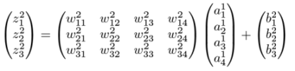
The activations in layer two are then obtained by applying σ to every entry of the resulting vector. This is nothing more than a notational simplification, but it is useful psychologically to pull out the numbers w_ij^l and b_j^l into their own matrices. These are the numbers that define the neural network itself, as opposed to the activations a jl that are the incremental steps in the evaluation.

To see what I mean, you can compare evaluating a neural network to evaluating the function f(x) = ax + b. The input variable is x, and by contrast, a and b are the constants that define the function; the space of possible linear functions is defined by the choice of a and b. The quantity ax, even if we relabeled it something like q, is merely an incremental step in the calculation of f(x). The analogy is that, once you’ve decided the number of neurons per layer in your MLP, the matrices of weights and vectors of biases for each layer are really the data defining the neural network. With that in mind, we can implement the MLP in Python.

16.3.5 Exercises

16.4 Building a neural network in Python

In this section, I show you how to take the procedure for evaluating an MLP that I explained in the last section and implement it in Python. Specifically, we’ll implement a Python class called MLP that stores weights and biases (randomly generated at first), and provides an evaluate method that takes a 64-dimensional input vector and returns the output 10-dimensional vector. This code is a somewhat rote translation of the MLP design I described in the last section into Python, but once we’re done with the implementation, we can test it at the task of classifying handwritten digits.

As long as the weights and biases are randomly selected, it probably won’t do better than the random classifier we built to start with. But once we have the structure of a neural network to predict for us, we can tune the weights and biases to make it more predictive. We’ll turn to that problem in the next section.

16.4.1 Implementing an MLP class in Python

If we want our class to represent an MLP, we need to specify how many layers we want and how many neurons we want per layer. To initialize our MLP with the structure we want, our constructor can take a list of numbers, representing the number of neurons in each layer.

The data we need to evaluate the MLP are the weights and biases for every layer after the input layer. As we just covered, we can store the weights as a matrix (a NumPy array) and the biases as a vector (also a NumPy array). To start, we can use random values for all of the weights and biases, and then when we train the network, we can gradually replace these values with more meaningful ones.

Let’s quickly review the dimensions of the weight matrices and bias vectors that we want. If we pick a layer with m neurons, and the previous layer has n neurons, then our weights describe the linear part of the transformation from an n -dimensional vector of activations to an m -dimensional vector of activations. That’s described by an m -by- n matrix, in other words, one with m rows and n columns. To see this, we can return to the example from section 16.3, where the weights connecting a layer with four neurons to a layer with three neurons made up a 4-by−3 matrix as shown in figure 16.15.

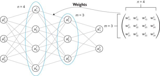
Figure 16.15 The weight matrix connecting a four neuron layer to a three neuron layer is a 3-by−4 matrix.

The biases for a layer of m neurons simply make up a vector with m entries, one for each neuron. Now that we’ve reminded ourselves how to find the size of the weight matrix and bias vector for each layer, we’re ready to have our class constructor create them. Notice that we iterate over layer_sizes[1:], which gives us the sizes of layers in the MLP, skipping the input layer which comes first:

class MLP():
    def __init__(self,layer_sizes):                 ❶
        self.layer_sizes = layer_sizes
        self.weights = [
            np.random.rand(n,m)                     ❷
            for m,n in zip(layer_sizes[:−1],
                           layer_sizes[1:])         ❸
        ]
        self.biases = [np.random.rand(n) 
                       for n in layer_sizes[1:]]    ❹

❶ Initializes the MLP with a list of layer sizes, giving the number of neurons for each layer

❷ The weight matrices are n-by-m matrices with random entries ...

❸ ... where m and n are the number of neurons of adjacent layers in the neural network.

❹ The bias for each layer (skipping the first) is a vector with one entry per neuron in the layer.

With this implemented, we can double-check that a two-layer MLP has exactly one weight matrix and one bias vector, and the dimensions match. Let’s say the first layer has two neurons and the second layer has three neurons. Then we can run this code:

>>> nn = MLP([2,3])
>>> nn.weights
[array([[0.45390063, 0.02891635],
        [0.15418494, 0.70165829],
        [0.88135556, 0.50607624]])]
>>> nn.biases
[array([0.08668222, 0.35470513, 0.98076987])]

This confirms that we’ve a single 3-by−2 weight matrix and a single 3D bias vector, both populated with random entries.

The number of neurons in the input layer and output layer should match the dimensions of vectors we want to pass in and receive as output. Our problem of image classification calls for a 64D input vector and a 10D output vector. For this chapter, I stick with a 64-neuron input layer, a 10-neuron output layer, and a single 16-neuron layer in between. There is some combination of art and science to picking the right number of layers and layer sizes to get a neural network to perform well on a given task, and that’s the kind of thing machine learning experts get paid big bucks for. For the purpose of this chapter, I say this structure is sufficient to get us a good, predictive model.

Our neural network can be initialized as MLP([64,16,10]), and it is much bigger than any of the ones we’ve drawn so far. Figure 16.16 shows what it looks like.

Figure 16.16 An MLP with three layers of 64, 16, and 10 neurons, respectively

Fortunately, once we implement our evaluation method, it’s no harder for us to evaluate a big neural network than a small one. That’s because Python does all of the work for us!

16.4.2 Evaluating the MLP

An evaluation method for our MLP class should take a 64D vector as input and return a 10D vector as output. The procedure to get from the input to the output is based on calculating the activations layer-by-layer from the input layer all the way to the output layer. As you’ll see when we discuss backpropagation, it’s useful to keep track of all of the activations as we go, even for the hidden layers in the middle of the network. For that reason, I’ll build the evaluate function in two steps: first, I’ll build a method to calculate all of the activations, and then I’ll build another one to pull the last layer activation values and produce the results.

I call the first method feedforward, which is a common name for the procedure of calculating activations layer-by-layer. The input layer activations are given, and to get to the next layer, we need to multiply the vector of these activations by the weight matrix, add the next layer biases, and pass the coordinates of the result through the sigmoid function. We repeat this process until we get to the output layer. Here’s what it looks like:

class MLP():
    ...
    def feedforward(self,v):
        activations = []                            ❶
        a = v
        activations.append(a)                       ❷
        for w,b in zip(self.weights, self.biases):  ❸
            z = w @ a + b                           ❹
            a = [sigmoid(x) for x in z]             ❺
            activations.append(a)                   ❻
        return activations

❶ Initializes with an empty list of activations

❷ The first layer activations are exactly the entries of the input vector; we append those to the list of activations.

❸ Iterates over the layers with one weight matrix and bias vector per layer

❹ The vector z is the matrix product of the weights with the previous layer activations plus the bias vector.

❺ Takes the sigmoid function of every entry of z to get the activation

❻ Adds the new computed activation vector to the list of activations

The last layer activations are the results we want, so an evaluate method for the neural network simply runs the feedforward method for the input vector and then extracts the last activation vector like this:

class MLP():
    ...
    def evaluate(self,v):
        return np.array(self.feedforward(v)[−1])

That’s it! You can see that the matrix multiplication saved us a lot of loops over neurons we’d otherwise be writing to calculate the activations.

16.4.3 Testing the classification performance of an MLP

With an appropriately sized MLP, it can now accept a vector for a digit image and output a result:

>>> nn = MLP([64,16,10])
>>> xv  = np.matrix.flatten(digits.images[0]) / 15.
>>> nn.evaluate(v)
array([0.99990572, 0.9987683 , 0.99994929, 0.99978464, 0.99989691,
       0.99983505, 0.99991699, 0.99931011, 0.99988506, 0.99939445])

That’s passing in a 64-dimensional vector representing an image and returning a 10-dimensional vector as an output, so our neural network is behaving as a correctly shaped vector transformation. Because the weights and biases are random, these numbers should not be a good prediction of what digit the image is likely to be. (Incidentally, the numbers are all close to 1 because all of our weights, biases, and input numbers are positive, and the sigmoid sends big positive numbers to values close to 1.) Even so, there is a biggest entry in this output vector, which happens to be the number at index 2. This (incorrectly) predicts that image 0 in the data set represents the number 2.

The randomness suggests that our MLP only guesses 10% of the answers correctly. We can confirm this with a test_digit_classify function. For the random MLP I initialized, it gave exactly 10%:

>>> test_digit_classify(nn.evaluate)
0.1

This may not seem like much progress, but we can pat ourselves on the back for getting the classifier working, even if it’s not good at its task. Evaluating a neural network is much more involved than evaluating a simple function like f(x) = ax + b, but we’ll see the payoff soon as we train the neural network to classify images more accurately.

16.4.4 Exercises

16.5 Training a neural network using gradient descent

Training a neural network might sound like an abstract concept, but it just means finding the best weights and biases that makes the neural network do the task at hand as well as possible. We can’t cover the whole algorithm here, but I show you how it works conceptually and how to use a third-party library to do it automatically. By the end of this section, we’ll have adjusted the weights and biases of our neural network to predict which digit is represented by an image to a high degree of accuracy. We can then run it through test_digit_classify again and measure how well it does.

16.5.1 Framing training as a minimization problem

In the previous chapters for a linear function ax + b or a logistic function σ(ax + by + c), we created a cost function that measured the failure of the linear or logistic function, depending on the constants in the formula, to match the data exactly. The constants for the linear function were the slope and y -intercept a and b, so the cost function had the form C(a, b). The logistic function had the constants a, b, and c(to be determined), so its cost function had the form C(a, b, c). Internally, both of these cost functions depended on all of the training examples. To find the best parameters, we’ll use gradient descent to minimize the cost function.

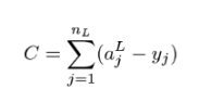
The big difference for an MLP is that its behavior can depend on hundreds or thousands of constants: all of its weights w_ij¹and biases b_j^l for every layer l and valid neuron indices i and j. Our neural network with 64, 16, and 10 neurons and its three layers have 64 · 16 = 1,024 weights between the first two layers and 16 · 10 = 160 weights between the second two. It has 16 biases in the hidden layer and 10 biases in the output layer. All in all, that’s 1,210 constants we need to tune. You can picture our cost function as a function of these 1,210 values, which we need to minimize. If we write it out, it would look something like this:

In the equation, where I’ve written the ellipses, there are over a thousand more weights and 24 more biases I didn’t write out. It’s worth thinking briefly about how to create the cost function, and as a mini-project, you can try implementing it yourself.

Our neural network outputs vectors, but we consider the answer to the classification problem to be the digit represented by the image. To resolve this, we can think of the correct answer as the 10-dimensional vector that a perfect classifier would have as output. For instance, if an image clearly represents the digit 5, we would like to see 100% certainty that the image is a 5 and 0% certainty that the image is any other digit. That means a 1 in the fifth index and 0’s elsewhere (figure 16.17).

Figure 16.17 Ideal output from a neural network: 1.0 in the correct index and 0.0 elsewhere

Just as our previous attempts at regression never fit the data exactly, neither will our neural network. To measure the error from our 10-dimensional output vector to the ideal output vector, we can use the square of their distance in 10 dimensions.

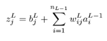
Suppose the ideal output is written y = (y₁ , y₁ , y₂ , ..., y₁₀ ). Note that I’m following the math convention for indexing from 1 rather than the Python convention of indexing from 0. That’s actually the same convention I used for neurons within a layer, so the output layer (layer two) activations are indexed (a₁² , a₂² , a₃² ,..., a₁₀¹).The squared distance between these vectors is the sum:

As another potentially confusing point, the superscript 2 above the a values indicates the output layer is layer two in our network, while the 2 outside the parentheses means squaring the quantity. To get a total cost relative to the data set, you can evaluate the neural network for all of the sample images and take the average squared distance. At the end of the section, you can try the mini-project for implementing this yourself in Python.

16.5.2 Calculating gradients with backpropagation

With the cost function C(w₁₁¹ ,w₁₂¹ , ..., b₁¹ , b₂¹ , ...) coded in Python, we could write a 1,210-dimensional version of gradient descent. This would mean taking 1,210 partial derivatives in each step to get a gradient. That gradient would be the 1,210-dimensional vector of the partial derivatives at the point, having this form

Estimating so many partial derivatives would be computationally expensive because each would require evaluating C twice to test the effect of tweaking one of its input variables. In turn, evaluating C requires looking at every image in the training set and passing it through the network. It might be possible to do this, but the computation time would be prohibitively long for most real-world problems like ours.

Instead, the best way to calculate the partial derivatives is to find their exact formulas using methods similar to those we covered in chapter 10. I won’t completely cover how to do this, but I’ll give you a teaser in the last section. The key is that while there are 1,210 partial derivatives to take, they all have the form:

or

for some choice of indices l, i, and j. The algorithm of backpropagation calculates all of these partial derivatives recursively, working backward from the output layer weights and biases, all the way to layer one.

If you’re interested in learning more about backpropagation, stay tuned for the last section of the chapter. For now, I’ll turn to the scikit-learn library to calculate costs, carry out backpropagation, and complete the gradient descent automatically.

16.5.3 Automatic training with scikit-learn

We don’t need any new concepts to train an MLP with scikit-learn; we just need to tell it to set up the problem the same way we have and then find the answer. I won’t explain everything the scikit-learn library can do, but I will step you through the code to train the MLP for digit classification.

The first step is to put all of our training data (in this case, the digit images as 64-dimensional vectors) into a single NumPy array. Using the first 1,000 images in the data set gives us a 1,000-by−64 matrix. We’ll also put the first 1,000 answers in an output list:

x = np.array([np.matrix.flatten(img) for img in digits.images[:1000]]) / 15.0
y = digits.target[:1000]

Next, we use the MLP class that comes with scikit-learn to initialize an MLP. The sizes of the input and output layers are determined by the data, so we only need to specify the size of our single hidden layer in the middle. Additionally, we include parameters telling the MLP how we want it to be trained. Here’s the code:

from sklearn.neural_network import MLPClassifier

mlp = MLPClassifier(hidden_layer_sizes=(16,),  ❶
                    activation='logistic',     ❷
                    max_iter=100,              ❸
                    verbose=10,                ❹
                    random_state=1,            ❺
                    learning_rate_init=.1)     ❻

❶ Specifies that we want a hidden layer with 16 neurons

❷ Specifies that we want to use logistic (ordinary sigmoid) activation functions in the network

❸ Sets the maximum number of gradient descent steps to take in case there are convergence issues

❹ Selects that the training process provides verbose logs

❺ Initializes the MLP with random weights and biases

❻ Decides the learning rate or what multiple of the gradient to move in each iteration of the gradient descen

Once this is done, we can train the neural network to the input data x and corresponding output data y in one line:

mlp.fit(x,y)

When you run this line of code, you’ll see a bunch of text print in the terminal window as the neural network trains. This logging shows how many gradient descent steps it takes and the value of the cost function, which scikit-learn calls “loss” instead of “cost.”

Iteration 1, loss = 2.21958598
Iteration 2, loss = 1.56912978
Iteration 3, loss = 0.98970277
...
Iteration 58, loss = 0.00336792
Iteration 59, loss = 0.00330330
Iteration 60, loss = 0.00321734
Training loss did not improve more than tol=0.000100 for two consecutive epochs. Stopping.

At this point, after 60 iterations of gradient descent, a minimum has been found and the MLP is trained. You can test it on image vectors using the _predict method. This method takes an array of inputs, meaning an array of 64-dimensional vectors, and returns the output vectors for all of them. For instance, mlp._predict(x) gives the 10-dimensional output vectors for all 1,000 image vectors stored in x. The result for the zero^th training example is the zero^th entry of the result:

>>> mlp._predict(x)[0]
array([9.99766643e-01, 8.43331208e−11, 3.47867059e-06, 1.49956270e-07,
       1.88677660e-06, 3.44652605e-05, 6.23829017e-06, 1.09043503e-04,
       1.11195821e-07, 7.79837557e-05])

It takes some squinting at these numbers in scientific notation, but the first one is 0.9998, while the others are all less than 0.001. This correctly predicts that the zero^th training example is a picture of the digit 0. So far so good!

With a small wrapper, we can write a function that uses this MLP to do one prediction, taking a 64-dimensional image vector and outputting a 10-dimensional result. Because scikit-learn’s MLP works on collections of input vectors and produces arrays of results, we just need to put our input vector in a list before passing it to mlp._predict :

def sklearn_trained_classify(v):
    return mlp._predict([v])[0]

At this point, the vector has the correct shape to have its performance tested by our test_digit_classify function. Let’s see what percentage of the test digit images it correctly identifies:

>>> test_digit_classify(sklearn_trained_classify)
1.0

That’s an astonishing 100% accuracy! You might be skeptical of this result; after all, we’re testing on the same data set that the neural network used to train. In theory, when storing 1,210 numbers, the neural net could have just memorized every example in the training set. If you test the images the neural network hasn’t seen before, you’ll see this isn’t the case; it still does an impressive job classifying the images correctly as digits. I found that it had 96.2% accuracy on the next 500 images in the data set, and you can test this yourself in an exercise.

16.5.4 Exercises

def test_digit_classify(classifier,start=0,test_count=1000):
    correct = 0
    end = start + test_count                           ❶
    for img, target in zip(digits.images[start:end], 
digits.target[start:end]):                             ❷
        v  = np.matrix.flatten(img) / 15
        output = classifier(v)
        answer = list(output).index(max(output))
        if answer == target:
            correct += 1
    return (correct/test_count)

>>> test_digit_classify(sklearn_trained_classify,start=1000,test_count=500)
0.962

def y_vec(digit):
    return np.array([1 if i == digit else 0 for i in range(0,10)])

def cost_one(classifier,x,i):
    return sum([(classifier(x)[j] − y_vec(i)[j])**2 for j in range(10)])

def total_cost(classifier):
    return sum([cost_one(classifier,x[j],y[j]) for j in range(1000)])/1000.

>>> total_cost(nn.evaluate)
8.995371023185067
>>> total_cost(sklearn_trained_classify)
5.670512721637246e-05

>>> nn = MLP([64,16,10])
>>> nn.weights = [w.T for w in mlp.coefs_]       ❶
>>> nn.biases = mlp.intercepts_                  ❷
>>> test_digit_classify(nn.evaluate,
                        start=1000,
                        test_count=500) 0.962    ❸

16.6 Calculating gradients with backpropagation

This section is completely optional. Frankly, because you know how to train an MLP using scikit-learn, you’re ready to solve real-world problems. You can test neural networks of different shapes and sizes on classification problems and experiment with their design to improve classification performance. Because this is the last section in the book, I wanted to give you some final, challenging (but doable!) math to chew on−calculating partial derivatives of the cost function by hand.

The process of calculating partial derivatives of an MLP is called backpropagation because it’s efficient to start with the weights and biases of the last layer and work backwards. Backpropagation can be broken into four steps: calculating the derivatives with respect to the last layer weights, last layer biases, hidden layer weights, and hidden layer biases. I’ll show you how to get the partial derivatives with respect to the weights in the last layer, and you can try running with this approach to do the rest.

16.6.1 Finding the cost in terms of the last layer weights

Let’s call the index of the last layer of the MLP L. That means that the last weight matrix consists of the weights w_ij^L ,where l = L, in other words, the weights w_ij^L .The biases in this layer are b jL and the activations are labeled a_j^L .

The formula to get the j^th neuron’s activation in the last layer a_j^L is a sum of the contribution from every neuron in layer L − l, indexed by i. In a made-up notation, it becomes

The sum is taken over all values of i from one to the number of neurons in layer L − l. Let’s write the number of neurons in layer l as ni, with i ranging from l to n_L−1 in our sum. In proper mathematical summation notation, this sum is written:

The English translation of this formula is “fixing values of L and j by adding up the values of the expression w_ij^L a_i^L−1 for every i from one to n_L.” This is nothing more than the formula for matrix multiplication written as a sum. In this form, the activation is as follows:

Given an actual training example, we can have some ideal output vector y with a 1 in the correct slot and 0’s elsewhere. The cost is the squared distance between the activation vector a_j^L and the ideal output values y_j. That is,

The impact of a weight w_ij^L on C is indirect. First, it is multiplied by an activation from the previous layer, added to the bias, passed through a sigmoid, and then passed through the quadratic cost function. Fortunately, we covered how to take derivatives of compositions of functions in chapter 10. This example is a bit more complicated, but you should be able to recognize it as the same chain rule we saw before.

16.6.2 Calculating the partial derivatives for the last layer weights using the chain rule

Let’s break it down into three steps to get from w_ij^L to C. First, we can calculate the value to be passed into the sigmoid, which we called z_j^L earlier in the chapter:

Then we can pass z_j^L into the sigmoid function to get the activation a_j^L :

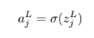
And finally, we can compute the cost:

To find the partial derivative of C with respect to w_ij^L ,we multiply the derivatives of these three “composed” expressions together. The derivative of z_j^L with respect to one particular w_ij^L is the specific activation a_j^L ₋₁ that it’s multiplied by. This is similar to the derivative of y(x) = ax with respect to x, which is the constant a. The partial derivative is

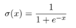
The next step is applying the sigmoid function, so the derivative of a_j^L with respect to z_j^L is the derivative of σ. It turns out, and you can confirm this as an exercise, that the derivative of σ(x) is σ(x)(1 − σ(x)). This nice formula follows in part from the fact that ex is its own derivative. That gives us

This is an ordinary derivative, not a partial derivative, because a_j^L is a function of only one input: z_j^L. Finally, we need the derivative of C with respect to a_j^L . Only one term of the sum depends on w_ij^L ,so we just need the derivative of (a_j^L − y_j)² with respect to a_j^L .In this context, y_j is a constant, so the derivative is 2a_j^L . This comes from the power rule, telling us that if f(x) = x² , then f'(x) = 2x. For our last derivative, we need

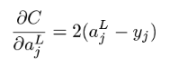
The multivariable version of the chain rule says the following:

This looks a little bit different from the version we saw in chapter 10, which covered only composition of two functions of one variable. The principle is the same here though: with C written in terms of a_j^L , a_j^L written in terms of z_j^L,and z_j^L written in terms of w_ij^L ,we have C written in terms of w_ij^L .What the chain rule says is that to get the derivative of the whole chain, we multiply together the derivatives of each step. Plugging in the derivatives, the result is

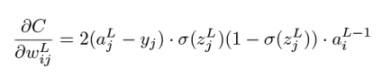
This formula is one of the four we need to find the whole gradient of C. Specifically, this gives us the partial derivative for any weight in the last layer. There are 16 × 10 of these, so we’ve covered 160 of the 1,210 total partial derivatives we need to have the complete gradient.

The reason I’ll stop here is because derivatives of other weights require more complicated applications of the chain rule. An activation influences every subsequent activation in the neural network, so every weight influences every subsequent activation. This isn’t beyond your capabilities, but I feel I’d owe you a better explanation of the multivariable chain rule before digging in. If you’re interested in going deeper, there are excellent resources online that walk through all the steps of backpropagation in gory detail. Otherwise, you can stay tuned for the (fingers crossed) sequel to this book. Thanks for reading!

16.6.3 Exercises

>>> from sympy import *
>>> X = symbols('x')
>>> diff(1 / (1+exp(-X)),X)
exp(-x)/(1 + exp(-x))**2

Summary

• An artificial neural network is a mathematical function whose computation mirrors the flow of signals in the human brain. As a function, it takes a vector as input and returns another vector as output.

• A neural network can be used to classify vector data: for instance, images converted to vectors of grayscale pixel values. The output of the neural network is a vector of numbers that express confidence that the input vector should be classified in any of the possible classes.

• A multilayer perceptron (MLP) is a particular kind of artificial neural network consisting of several ordered layers of neurons, where the neurons in each layer are connected to and influenced by the neurons in the previous layer. During evaluation of the neural network, each neuron gets a number that is its activation. You can think of an activation as an intermediate yes-or-no answer on the way to solving the classification problem.

• To evaluate a neural network, the activations of the first layer of neurons are set to the entries of the input vector. Each subsequent layer of activations is calculated as a function of the previous layer. The final layer of activations is treated as a vector and returned as the result vector of the calculation.

• The activation of a neuron is based on a linear combination of the activations of all neurons in the previous layer. The coefficients in the linear combination are called weights. Each neuron also has a bias, a number which is added to the linear combination. This value is passed through a sigmoid function to get the activation function.

• Training a neural network means tuning the values of all of the weights and biases so that it performs its task optimally. To do this, you can measure the error of the neural network’s predictions relative to actual answers from a training data set with a cost function. With a fixed training data set, the cost function depends only on the weights and biases.

• Gradient descent allows us to find the values of weights and biases that minimize the cost function and yield the best neural network.

• Neural networks can be trained efficiently because there are simple, exact formulas for the partial derivatives of the cost function with respect to the weights and biases. These are found using an algorithm called backpropagation, which in turn makes use of the chain rule from calculus.

• Python’s scikit-learn library has a built in MLPClassifer class that can automatically be trained on classified vector data.