Introduction to photovoltaic system performance
N.M. Pearsall Northumbria University, Newcastle upon Tyne, United Kingdom
Abstract
Photovoltaic systems are used in a wide range of applications and can be designed in a range of configurations, including grid-connected or stand-alone, fixed or tracking, flat plate or concentrator operation. This chapter discusses the basic components and designs of the photovoltaic system and describes the performance parameters used to express the system output. It provides an introduction to the principles of photovoltaic system performance for those new to the technology, a reminder for the more experienced readers and a basis for the more in-depth discussions in the later chapters of the book.
Keywords
Grid-connected PV systems; Stand-alone PV systems; PV system efficiency; Performance ratio; PV module technology; Inverter; PV design principles
1.1 Introduction
Photovoltaic (PV) systems, which convert solar irradiation directly to electricity, can be used for a wide range of applications, from small systems powering loads such as sensors or domestic lighting through to large systems feeding electrical power directly into the electricity grid. Despite this variety of uses, the basic system configuration is rather simple. The heart of the system is the PV array itself, a collection of PV modules totalling the required power capacity of the system. The balance of system (BOS) components then include equipment for power conditioning and energy storage, mounting and support of the array, measurement of system performance and safety assurance.
The performance of the system, which mainly concerns the energy output, both in quantity and in timing, depends on the operating conditions and the detailed configuration of the system. In turn, the operating conditions depend on the location of the system, which governs the solar irradiation received, the ambient temperature and other climate-related aspects that influence the system performance. How the system performs determines its technical and economic feasibility and whether it is the best solution in terms of a source of electricity for any given application.
This chapter provides an introduction to the configuration of PV systems, what influences their performance and how that performance is expressed. It is intended for readers who are unfamiliar with PV systems, but can also be used as a summary chapter for those who want to refresh their knowledge about the systems. It provides a foundation for the later chapters in this book, which consider various aspects of system performance in greater detail.
1.2 The PV system
1.2.1 System categories
PV systems can be classified into two main categories, depending on whether or not they are connected to the local electricity network (or grid). Grid-connected systems are generally designed to produce their maximum energy output at all times and to contribute to meeting electrical loads, either close to the system (generally termed local loads) or via the electricity network. Stand-alone PV systems operate independently from the grid supply and are often located where there is no electricity grid or the grid is difficult to access. In this case, the system is designed to supply the required amount of electricity for the specified load, but does not always necessarily provide the maximum output from the system. This is discussed further in Section 1.3, in terms of expressing these differences in performance mode.
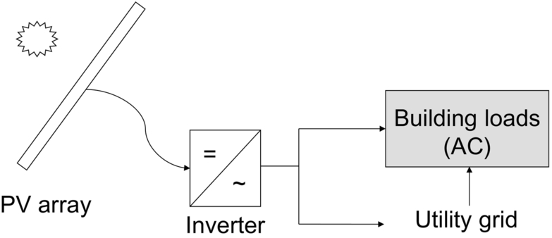
Grid-connected PV systems accounted for around 99% of the cumulative capacity installed worldwide at the end of 2014, according to the International Energy Agency Photovoltaic Power Systems Programme (IEA PVPS) [1], and the market in 2015 is expected to have been similarly dominated by this system category. The concept of the grid-connected PV system is simple and is shown schematically in Fig. 1.1. The PV array is connected to an inverter, which converts the DC output of the array into AC output matching the voltage and frequency of the local grid supply. The system can be connected in parallel with the grid and used to meet local loads. In this case, the output from the PV system will be fed to the load and any shortfall will be supplied from the grid. If there is an excess of generation from the PV system, this excess will be exported to the grid. Alternatively, if there are no significant local loads to be met, the entire output of the PV system may be fed into the grid. It should be noted that the system shown in the figure does not include any facility for the storage of electricity and this is the usual configuration of most current grid-connected systems. However, as the penetration of PV systems on the grid increases and, in some cases, for economic reasons related to the value of local use of electricity, there is a growing interest in storage, either local or central, for grid-connected systems and it can be expected that this will become more common in the future.
The grid-connected system is often classified into distributed and centralized systems, but there are different definitions in regard to how this classification is made. The definition can be made in regard to size (eg, small systems less than, say, 100 kW in capacity would be classed as distributed, whilst larger systems would be considered as centralized), configuration (eg, those meeting local loads are distributed, those only feeding into the grid are centralized) or grid connection point (eg, systems connected to the low voltage distribution feeder are classed as distributed, those connected at a higher voltage are centralized). The IEA PVPS defines distributed (or decentralized) systems in terms of their function being to meet the needs of a specified customer or group of customers, whereas centralized systems feed into the general grid supply. Their data show that distributed systems represented around 56% of the cumulative installed capacity at the end of 2014 [1]. Building-related systems, where the PV array is integrated into or attached to the roof or façade of a building to meet loads within that building, are typical examples of a distributed system.
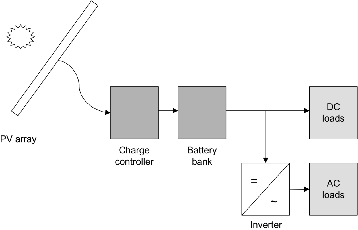
The stand-alone system operates independently from the grid and provides the only power source to meet a particular specified load, for example, telecommunications mast, water pumping, medical refrigeration and many more. The most common configuration of the system comprises the PV array, battery storage, a charge controller (to control the charging and discharging of the batteries and to provide maximum power point (MPP) tracking) and the specified load. This is shown schematically in Fig. 1.2. The load must form part of the design of the system, so as to ensure the PV array and battery storage are sized to meet the load under all relevant weather conditions. In some cases, particularly when there is a large variation of the load profile and/or a large seasonal variation in sunlight levels, a hybrid system is used, where this includes one or more additional electricity generation technologies (eg, wind turbine, diesel generator).
PV systems can be classified as either flat plate or concentrator systems. In the latter, optical components, namely lenses or mirrors, are used to increase the intensity of the sunlight falling on the PV devices. Concentrator systems can be further classified into low concentration (up to 30 ×) and high concentration (> 300 ×) and require the modules to be moved to track the sun, since it is only possible to optically concentrate direct sunlight. Flat plate PV arrays can also be operated in sun-tracking mode, if desired and where the application allows.
When considering the performance of the system, it is clear that the operating mode, in terms of connection options, concentration level and static/tracking options, must be considered in determining the expected values.
1.2.2 PV module technologies
A range of semiconductor materials could be used in PV modules, but to achieve commercial viability, the modules have to have a suitably high performance coupled with stability in operation, have good manufacturability, have low cost production and be able to achieve a long lifetime. Manufacturability includes aspects such as ease of manufacture, availability of materials, health and safety, environmental impacts, reproducibility and yield. The current flat plate market is dominated by crystalline silicon, both monocrystalline and multicrystalline, with the latter having the highest market share. In 2014, crystalline silicon modules are estimated to have accounted for almost 91% of the PV market, with multicrystalline silicon contributing 55% and monocrystalline silicon 36% [2]. Other commercial flat plate technologies include cadmium telluride (CdTe), copper indium gallium diselenide (CIGS), amorphous silicon (a-Si) and several hybrid designs incorporating crystalline, nanocrystalline and a-Si (eg, heterojunction with intrinsic thin layer cells, micromorph cells). Organic and polymer based cells have seen rapid developments over recent years, although are not yet utilized in the power market. In the concentrator market, low concentration systems use silicon technology whereas the high concentration systems are based on high efficiency multijunction cells utilizing various III–V compound materials (eg, GaInAs/GaInP/Ge triple junction cells). For a more in-depth discussion of the status of current and emerging PV cell technologies, see, for example, the recently published study by MIT on the future of solar energy [3].
In terms of performance, the most obvious difference between the module types is the rated conversion efficiency, that is, the ratio between the electrical output of the module and the solar irradiation received under specified operating conditions (see Section 1.3.3 for a full definition). However, there is also variation in the voltage and current parameters, with both parameters being a function of the energy bandgap of the semiconductor material used for the absorber layer of the PV device. Thus, for example, the voltage per cell of a CdTe device is higher than for a silicon device, due to the higher bandgap of the CdTe material, but the current density is lower (under the same operating conditions for both devices).
There is continual development of module designs and production methods, leading to an increase in efficiency over time. Also, whilst it is straightforward to find the highest reported laboratory cell or small module efficiencies at any given time, the average efficiency of commercial modules is more difficult to establish. According to the status report by the Fraunhofer Institute for Solar Energy Systems published in 2015 [2], the efficiency ranges of commercial PV modules are as shown in Table 1.1.
Table 1.1
Efficiency ranges for commercial PV modules—reported values by Nov. 2015
| Module technology | Efficiency range under standard test conditionsa (%) | Highest reported laboratory efficiency (module) (%) |
| Monocrystalline silicon | 16–19 | 22.9 |
| Multicrystalline silicon | 15–17 | 18.9 |
| Thin-film CdTe and CIGS | 14–15 | 17.5 |
| Advanced silicon designs (heterojunction, interdigitated back contact, etc.) | 18–21 | Not available (best cell efficiency of 25.6%) |
| Concentrator (> 400 ×)b | 27–33 | 38.9 |
Adapted from data presented in Fraunhofer Institute for Solar Energy Systems, Photovoltaics report, http://www.ise.fraunhofer.de, November 2015.
a See Section 1.3.2 for an explanation of standard test conditions (STC).
b Note that the STC for concentrator modules differ from those for flat plate modules, as discussed in Section 1.3.2.
Other module parameters that lead to a difference in module performance include spectral response (the dependence of the output on the spectral content of the incident light), temperature coefficients for voltage, current and power, cell stability and variations in module design (eg, cell spacing, module materials). Whilst all of these can be determined for the module, care must be taken in both the measurement of these parameters and their use in determining module performance under conditions which differ from those used during measurement. For example, because the basic cell shape varies with technology (square or pseudo-square for crystalline silicon, long narrow strips for thin film), the electrical effect of shading may differ for the same shading pattern since a different number of cells will be affected (see Section 1.3.1 for more information on the effect of shading).
In general, the information in the rest of this chapter applies to all current commercial cell technologies, unless stated, although some special conditions apply to concentrator systems and readers are referred to Chapter 10 of this volume for a more in-depth discussion of their performance.
1.2.3 BOS equipment
The BOS equipment is generally defined as all the components of the system other than the PV array itself. This can include power conditioning (eg, inverter, DC–DC converter), electricity storage (eg, rechargeable battery), wiring, fuses and switches, monitoring equipment, etc., depending on the system details. It can be seen from the system schematic diagrams in Figs 1.1 and 1.2 that the BOS components depend on whether the system is grid connected or stand-alone, whether the loads to be met are AC or DC and whether the system includes any storage facility.
The main aim of the system design in terms of choice and specification of BOS components is to achieve the highest system efficiency possible for the choice of module. This may include both selecting the BOS components that are suitable for the system and modifying the PV array specifications to best match to the rest of the system (see Section 1.3.1 for further explanation of this aspect). Wiring cross-sections and cable lengths must be chosen for minimum energy loss, especially for low voltage systems.
Component efficiency can be expressed by the usual ratio of energy out to energy in, measured at the appropriate point in the system. The lifetime of the BOS components and any degradation characteristics must also be taken into account in determining the effect of the BOS equipment on system performance. The performance parameters of the main items of BOS equipment are discussed further in Section 1.3.4 and the effects of various system losses are considered in Section 1.3.3.
1.3 Expressing PV system performance
In this section, we will consider the main methods of expressing the performance of PV systems and their constituent parts of PV modules and BOS components. The performance parameters described are then used in later chapters in this book to provide a more detailed consideration of predicting and measuring the performance of a PV system.
1.3.1 Current–voltage and power–voltage characteristics
Most current commercial solar cells have the structure of a diode, a junction between p- and n-type semiconductor materials. In some cases, an insulating layer is introduced to create a p–i–n junction or a series of junctions are created. However, from the point of view of the electrical characteristics of the device, the behaviour is similar. The relationship between the current, I, and the voltage, V, can be expressed, in the ideal case, by the relationship given in Eq. (1.1). This is the standard diode equation, with the addition of the light generated current, IL, and a diode factor, n, which is related to the recombination mechanisms in the cell.

Here, I0 is the reverse saturation current of the diode, q is the charge on the electron (1.602 × 10− 19 C), k is Boltzmann's constant (1.38 × 10− 23 m2 kg/s2 K) and T is the temperature in kelvin. The parameters I0, IL and n are dependent on the cell materials and design.
For a real device, it is also necessary to include the resistances relating to carrier transport in the semiconductor material, the ohmic contacts at the front and rear of the cell and the bulk resistance of the semiconductor layers. These are often represented by two lumped resistances, known as the series resistance, Rs, and the shunt resistance, Rsh. Including these in the preceding equation results in the I–V characteristic of a real solar cell being represented by Eq. (1.2):
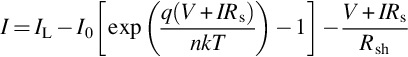
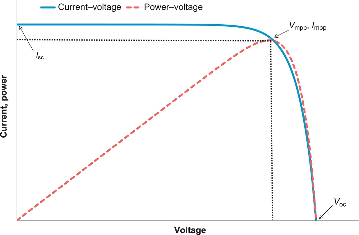
The resulting I–V characteristic is shown in Fig. 1.3, along with the power–voltage characteristic, where the power output, P, of the cell is determined from the usual relationship, P = I × V. The characteristic is shown for an arbitrary operating condition (see Section 1.3.2 for a discussion of the effect of operating conditions).
Eq. (1.2) applies to a variety of cell types and gives a good representation of the I–V relationship. In some cases, the cell is more closely represented by two diode expressions in the equation, each having different I0 and n values, but this consideration is beyond the scope of this chapter. Interested readers are referred to volumes dealing with the detailed analysis of solar cell structures [4]. Nevertheless, the two-diode model also leads to an I–V characteristic of the same general shape.
The I–V characteristic shown in Fig. 1.3 applies not only to the individual solar cells, but also to PV modules (a number of electrically connected PV cells, encapsulated into a single item) and to PV arrays (a collection of electrically connected PV modules). Clearly, there is some modification of the resistance values as we move from cells to modules to arrays, but the general shape of the characteristic remains. Thus, the following discussion applies equally to cells, modules and arrays.
The following parameters are generally used to describe the performance of the PV device, as illustrated in Fig. 1.3:
• Short circuit current, Isc—this is the current when there is zero resistance between the device terminals. It represents the maximum current for the specific operating conditions of the device.
• Open circuit voltage, Voc—this is the voltage across the device terminals in open circuit. It represents the maximum voltage for the specific operating conditions.
• MPP—the power level varies along the I–V characteristic and the MPP represents the point at which the power is the maximum value.
• Current at MPP, Impp—the current value at the position on the characteristic for which the I × V value is maximum.
• Voltage at MPP, Vmpp—the voltage value at the position on the characteristic for which the I × V value is maximum.
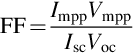
• Fill factor, FF—the ratio of the product of Impp and Vmpp to the product of Isc and Voc, as represented by Eq. (1.3).
The MPP is also used to define the efficiency of the device, which is given by the standard equation,
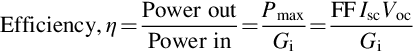
where Pmax = Impp × Vmpp and Gi is the incident global irradiance.
The PV device will operate at the point of the I–V characteristic where the relationship given by Ohm's Law is satisfied for the resistance of the load across the terminals, that is, at the point where R = V/I. In the ideal case, we would wish to be operating at the MPP, such that Rmpp = Vmmp/Impp. However, the values of the parameters that define the I–V characteristic are dependent on the operating conditions, particularly irradiance and operating temperature, and so the value of Rmpp will change as the conditions change. Therefore, most PV systems will include a maximum power point tracker (MPPT), which modifies the operating point on the I–V curve in order to operate for as much of the time as possible at the MPP.
The PV array is a collection of PV modules that are electrically connected, either in series or parallel connection. The choice of connections determines the voltage and current output of the array. Series connection (the positive terminal of one module connected to the negative terminal of the next) increases voltage, leaving the current equivalent to that of the single module. Parallel connection (positive terminals connected together, as are negative terminals) increases the current, whilst leaving the voltage the same as for a single module. By means of a combination of series and parallel connections, the required current and voltage outputs for the array can be achieved.
For best performance, it is important that the performance of all modules that are electrically connected is as uniform as possible. If the modules do not have uniform performance, then the voltage at the MPP will be different for different modules. Whilst it is possible to determine the MPP for the combined set of modules, each individual module will not be operating at its MPP and therefore this results in a loss of potential output. In practice, this means that electrically connected modules should be all of the same type and model, that their individual output characteristics should be as similar as possible and that they should be operating under the same conditions of irradiance and module temperature. This implies similar mounting systems and the same orientation (tilt angle and azimuth angle).
One of the most common sources of nonuniformity is shading of the array, although the system design should attempt to keep this as low as possible. If one module is shaded whilst the other modules to which it is connected are in sunlight, the shaded module can act as a load and may be damaged by localized heating due to high current levels. To protect the module, it is usual to incorporate one or more bypass diodes, through which the current is diverted to prevent the shaded cells drawing current. However, this results in a modification of the power–voltage curve and a loss of output. The loss can be minimized by separating shaded modules from unshaded modules in the connection design, so ensuring that the MPP tracking is performed on modules with similar performance levels, but this requires careful design in both the connections and the number of MPPTs used. There is a range of options for the configuration of modules and inverters, ranging from a single inverter serving the whole array (with one or more MPPTs) to inverters attached to single modules (so-called microinverters). The system design can also mix module level MPPTs with a single central inverter. The best system design depends on the extent of the nonuniformity on the array and the economic evaluation of each option.
1.3.2 Operating conditions
As has already been discussed, the output of a PV device is dependent on its operating conditions, in particular the solar irradiance and the operating temperature as can be seen from Eqs (1.1), (1.2). The output is also dependent on the solar spectrum, since the spectral response of the device varies with the absorber material used and the device structure. Therefore, in order to be able to compare performance, a standard set of operating conditions has been defined by the PV community for the measurement of PV cells and modules.
The standard test conditions (STC) are [5]
• AM1.5 standard global spectrum
• Operating temperature of 25°C
• Normal incidence irradiance
Note that these are the conditions for flat plate PV systems. A discussion of the testing conditions for concentrator PV modules can be found in Chapter 10.
The standard spectrum is defined for a specific path length through the atmosphere that is represented by the air mass (AM) number. The AM number can be calculated as 1/sin(α), where α is the solar altitude angle (the angle between the direct line to the sun and its projection on the horizontal, measured in the vertical plane). AM1 is the condition for a location at sea level with the sun directly overhead. In order to determine the spectrum, the atmospheric conditions must also be specified in order to determine the absorption and scattering of the sunlight. The standard global spectrum is given in the IEC standard 60904-3 [6].
These test conditions are suitable for the measurement of PV modules in the factory, since they do not require specific heating or cooling of the modules to achieve the required operating temperature. However, they do not represent the conditions that the module is likely to experience in practice, apart from under very specific circumstances. At the STC irradiance level of 1000 W/m2 and an ambient temperature consistent with a low altitude site (say, in the range of 10–40°C), then the module operating temperature will be considerably higher than the STC value of 25°C. The temperature of the module in an operating PV system depends on
• the irradiance level, since this is the energy input to the system,
• the construction of the module, especially in regard to heat transfer through the module and from the module surfaces,
• the module efficiency, since any solar energy not converted to electricity will be converted to heat,
• the mounting method, particularly in regard to the air flow around the module and
• the ambient temperature, wind speed and wind direction, which impact on the heat removal from the module.
In order to consider the difference in operating conditions in the field from those at STC, it is usual to also measure the nominal operating cell temperature (NOCT), which is determined from field measurements. Nevertheless, this is still only for one specific set of operating conditions, namely:
• Ambient temperature of 20°C
• Module is mounted on an open rack at an angle of 45 degrees
• Wind speed is 1 m/s
• Module at open circuit (no load)
The procedure is to measure the module temperature at several times during the test period when the conditions are close to those required and then extrapolate to the NOCT condition [5]. The NOCT value is usually provided in the module datasheet and is typically between 45°C and 50°C, although this will depend on module construction.
The NOCT value can be used directly to predict the module temperature for any combination of irradiance and ambient temperature, provided that the other system parameters are closely matched to the NOCT measurement conditions (ie, open rack mounting with good ventilation, low wind speed). The translation formula is given in Eq. (1.5):
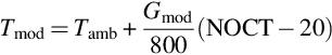
where Tmod is the module temperature, Tamb is the ambient temperature and Gmod is the global irradiance incident on the module. Nevertheless, the NOCT only represents module temperature for one specific set of conditions, even if these are more likely to represent operational conditions than do STC parameters. Therefore, it is useful to have a model for the prediction of module temperature under a range of conditions.
Eq. (1.5) can be rearranged to state that the difference between the module temperature and ambient temperature is proportional to irradiance and this has also been shown empirically, to at least a good approximation. Most module temperature models include this assumption, although there may also be other terms. The simplest concept is that originally proposed by Ross [7], as shown in Eq. (1.6):
where k is a constant which depends on the cell technology, the module construction, the mounting method and the environmental conditions. It should be noted that the preceding two relationships do not include thermal lag, which would have some influence on module temperature. Thus, more representative values are obtained for hourly average irradiance values than for instantaneous irradiance values. Other models include explicit terms for wind speed or are based on thermal transfer equations. An in-depth review of thermal models for the estimation of PV module temperatures has been published by Segado et al. [8].
The variation of PV module (or array) output with changes in operating conditions can be summarized as follows:
• The current has a linear relationship with irradiance level, whereas the voltage varies logarithmically due to the exponential term in the I–V equation.
• Current increases slightly with temperature, but the voltage reduces more strongly, leading to a reduction in power output with increasing temperature—the temperature coefficients for both current and voltage are dependent on the PV cell material and cell design.
• Power increases proportionally with irradiance and reduces with increasing temperature.
• The current is dependent on the spectral content of the incident sunlight and the properties of the absorber material.
For a practical PV system, the operating conditions will change consistently through the day, due to the change in sun position, temperature and weather conditions.
1.3.3 Efficiency, yield and performance ratio
The performance of a PV system is generally expressed by one of three parameters: the system efficiency, the energy yield or the performance ratio (PR). These parameters are linked but express different aspects of the overall performance.
The efficiency of the PV device, as represented by Eq. (1.4), has already been discussed and expresses how well the device converts the incoming solar energy to electricity. For a PV module, the efficiency is usually quoted under STC, although it will vary with operating conditions as described in the previous section. At the system level, we must include the efficiency of all other components in the system as well, to determine the overall system efficiency. Examples of this would be the inverter efficiency for the conversion of DC to AC electricity, any losses in the wiring, MPPT losses, etc. Clearly, the higher the system efficiency, the greater the output of the system for a given solar input and we would want to achieve the highest system efficiency that is reasonably practical for that system. However, the efficiency value depends directly on the efficiency of the PV array and therefore on the cell technology chosen, as well as some other design features of the module. Thus, it is difficult to compare absolute values of efficiency between systems of different technologies in order to determine information on system losses.
The energy yield of a system expresses the energy output and so is of particular interest to the system user. Three energy yield values have been defined, with, in each case, the energy output normalized to the PV array rating. The most useful of these is termed the final yield and represents the energy delivered to the load per unit capacity of the system. Note that, for a grid-connected system feeding power directly to the grid rather than to local loads, the final yield would be calculated using the energy to the grid.
Thus,
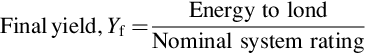
where the energy to load is often expressed in kilowatt hours and the system rating in kilowatts and the yield is calculated over a specified period, for example, annual. Since the output of the system is dependent on the solar energy input, the yield value will clearly be location dependent and it is possible to determine typical yields for different regions or countries. Yield values are also dependent on system details, such as the orientation of the array and whether or not tracking is used.
The second yield is known as the array yield, YA and is defined in a similar way to the final yield, but now using the energy output from the array only (ie, before conversion to AC in the inverter). This gives a measure of the performance of the array and can help to distinguish between operational issues relating to the array and to the BOS components. However, it is only possible to determine array yield if there is a measurement of the array output at the relevant point in the system.
The third yield value is known as the reference yield. This expresses the output of the system if there were no losses, that is, in the ideal case. Thus, it considers the case when the array operates continually under STC, there is perfect MPP tracking, the DC to AC conversion efficiency is 100%, etc. However, it does take into account the solar energy received by the system. Because the system rating, which appears in the denominator for all the yield calculations, is defined as the output under STC, we can determine reference yield from the following equation:
where GA is the irradiation received by the array over the period considered, expressed in kWh/m2, and GSTC is the STC irradiation, that is, 1 kWh/m2.
We have seen that the system efficiency is dependent on module choice and the final yield is dependent on the solar irradiation received, so making it difficult to use these values to determine performance quality without some benchmark of efficiency or yield for each system. The PR takes into account both system design and solar irradiation by comparing the final yield of the system with its reference yield. Thus,
As can be seen, the PR compares the actual yield achieved by the system to the yield in the ideal case and so provides a measure of the overall losses, and hence the quality, of the system. The PR value is widely used to allow comparison between systems and in the monitoring of performance over time, since changes in the PR value indicate a change in the system losses. In practice, the determination of PR requires only the measurement of energy output from the system and the solar irradiation received by the PV array over the defined period, together with knowledge of the nominal rating of the system.
We can define the following typical loss factors for a grid-connected PV system, starting with the losses at the array level and moving through the system components to the grid connection (note that the order does not imply the importance of the loss):
• Module operating temperature—expresses the difference in performance due to the module not operating at 25°C, usually a loss because the module temperature is higher but can be a gain in low temperature locations.
• Module rating—because the final yield is normalized to the array rating, it assumes that all modules achieve that rating. In practice, modules may have a higher or lower rating within the manufacturer specification and this will affect the value of PR calculated.
• Angle of incidence effects—STC requires irradiance at normal incidence, whereas in practice the irradiance is received at a range of incidence angles depending on module orientation and solar position. At high incidence angles, more light is reflected from the module surface and the absorption path of the light in the cell is changed, so leading to reduced output.
• Low light level effects—for some modules, the response reduces at low light levels (below 100 W/m2) and the inverter will also have reduced efficiency for low power levels.
• Module mismatch—if modules with different operating characteristics under STC are electrically connected, there will be a loss since it will not be possible to operate all the modules at their MPP for a given operating voltage. The magnitude of the loss depends on the level of mismatch and it is common to select modules so as to minimize the mismatch when designing the array.
• Shading—the shading of parts of the array results in both a loss of output due to the reduced output of the shaded modules and a loss due to the increase in the mismatch between shaded and unshaded modules. The extent of the loss depends on the degree of shading and the connection of modules in the array.
• Dirt or ice/snow accumulation—in both cases, the light transmitted into the module will be reduced and this will reduce the system output. The extent of the loss depends on the soiling (or snow) at the location and any maintenance activities implemented (eg, cleaning, clearing the snow).
• MPP tracking losses—as the operating conditions change, the MPP also changes and the tracker must then reacquire the MPP. The losses relate to the period spent away from the MPP whilst the tracker searches for the correct operating point and depend on the detailed algorithm used for the tracker and the rate of variation of conditions.
• Inverter efficiency—the efficiency of the inverter varies with input power, input voltage and the inverter design (eg, single or multistage, with or without transformer). Included here would be the efficiency of any power conditioning equipment (eg, DC to DC conversion) that is required for the particular system.
• Inverter threshold—inverters consume small amounts of power in the conversion and control processes and so there is a set threshold of output from the PV array below which the inverter will be shut down so that it does not draw more power from the grid than is being generated. The appropriate threshold depends on the inverter, with modern insulated-gate bipolar transistor-based inverters having a much lower required threshold than the older thyristor-based inverters.
• Cabling losses—all electrical systems have losses in the cables linking parts of the system and these are dependent on the voltage levels, cable cross-sectional area and cable length.
• Reliability of system components—any down time of system components that affects the magnitude of the system output will influence the PR value calculated.
• Reliability of grid connection—in most cases, the grid-connected PV system will be required to shut down if the local grid supply to which it is connected is out of specification in terms of voltage or frequency. The details of the conditions for shut down are specific to the connection regulations for the grid in question, but it is clear that any lack of reliability on the grid, even if unrelated to the PV system, may cause periods of no output and this will be reflected in the calculated PR value.
It can be seen from the preceding list that there are many factors that influence the PR value, but nevertheless it is the most useful of the three parameters to determine long-term performance. With knowledge of the system and, where necessary, the use of other measured parameters to allow quantification of some of the losses detailed here, it becomes possible to identify the system losses that can be addressed and so improve the system performance. When the PR value is used over time to indicate changes in system performance, it is important to make sure that the measurement equipment is reliable and the sensors are suitably calibrated (and cleaned in the case of the irradiance sensor). If measurement of the irradiation is not made on-site, it is possible to use satellite-derived values or measurements at a nearby site provided that it is sufficiently close to provide a meaningful value. In all cases, the accuracy of the values should be taken into account in determining the accuracy with which the PR value is known.
Since the module operating temperature is one of the strongest influences on module performance, it is generally possible to observe a seasonal variation of PR due to the change in ambient temperature across the year. Therefore, if the assessment of other losses is the main focus of the analysis, a temperature corrected PR value is sometimes used. This modifies the reference yield value to account for the variation of temperature from STC and thus allows the seasonal temperature variation to be removed from consideration. This allows the variation of other loss mechanisms to be seen more clearly in the analysis.
The discussion so far has considered grid-connected systems, but the same parameters of efficiency, yield and PR can also be calculated for stand-alone systems. However, since the stand-alone system is designed to meet a specific load, an inherent property of that design is that the system would be able to provide excess energy at some times of the year since it is required to meet load under the worst-case conditions. In practice, this means that the array will sometimes be operated away from MPP, so as to only produce the amount of energy required for the load. As a result, the yield will be limited to the load requirement and both efficiency and PR will be substantially lower than for the grid-connected system, which is designed for continuous MPPT operation. Indeed, for a stand-alone system that is designed to meet a critical load (such as health care or communications), the additional capacity that is needed to provide the required safety margin would lead to a reduction in the calculated PR value, so the PR cannot be taken as an indication of quality. The performance parameters that can be considered for a stand-alone system are discussed in the next section.
1.3.4 Other performance parameters
The three performance parameters discussed in the previous section express the overall performance of the system but it is sometimes useful to consider the specific performance of certain parts of the system in order to ensure the correct design and operational choices.
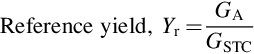
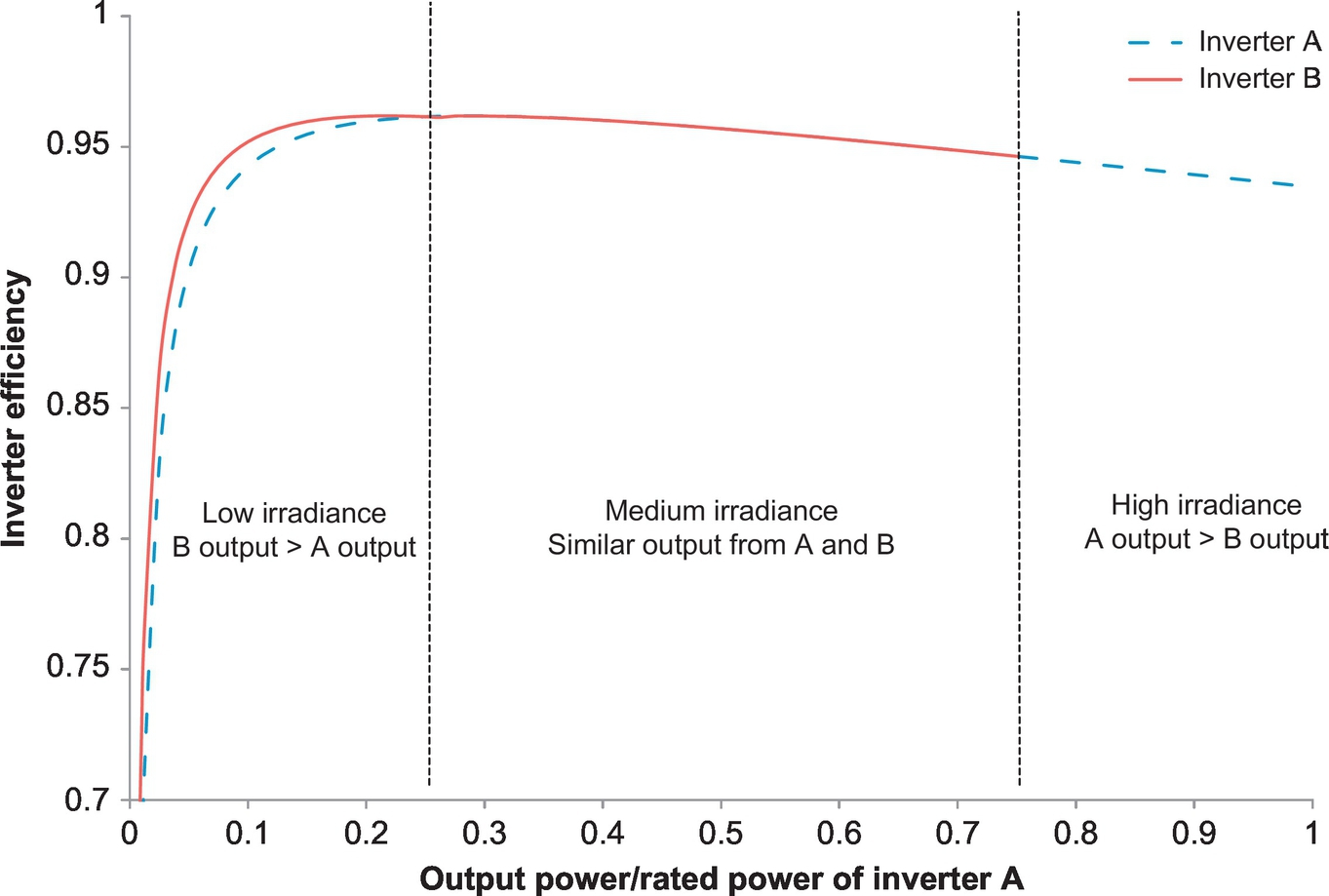
It is possible to determine the inverter efficiency if measurements of both DC input and AC output are provided. In general, the efficiency of a PV inverter is a function of the input power and input voltage, with a typical set of efficiency curves being shown in Fig. 1.4. At medium to high light levels and therefore input power from the array, the inverter has a high efficiency, generally well in excess of 90%. At low irradiance levels, the efficiency drops off sharply. This means that we can determine an optimum inverter capacity in comparison with the array capacity, such that the balance between energy loss at the low irradiance end due to reducing efficiency is balanced against energy loss at the high irradiance end due to limiting because of the maximum inverter capacity. This is illustrated in Fig. 1.5, assuming that the basic shape of the inverter efficiency curve does not depend on inverter capacity. Clearly, the balance between energy generation at low and high irradiance values is dependent on the climate and, therefore, so is the optimum inverter/array ratio, with the general approach of a reduction in this ratio as the latitude increases.
Because of the variation of efficiency with input power, and therefore irradiance on the array, the average operating efficiency of the inverter will vary with climate. In general, the technical information for a PV inverter will include both the peak efficiency (usually between 95% and 98% depending on the inverter technology) and a weighted efficiency to account for the operation at different irradiance levels. In Europe, this weighted efficiency is termed the Euro efficiency [9] and can be represented by Eq. (1.10), as follows:
Here, Eff@5% is the DC to AC conversion efficiency at an input power of 5% of the inverter capacity, with similar definitions for the other terms. The weighting reflects the amount of energy predicted to be gained at each energy level. An alternative weighting, using the same rationale and approach, is the California Energy Commission or CEC efficiency, calculated as follows [10]:
Here the weighting factors are more heavily biased towards the higher irradiance levels, to reflect the difference between the climates in the southwestern USA and central Europe. The use of either the Euro or CEC efficiency gives a lower but more representative value than the peak efficiency in terms of considering the overall inverter efficiency across a period of operation. Clearly, other weightings could be developed for other climate options, although there needs to be consensus within the community for widespread use.
For a stand-alone PV system, the important parameter is not the total energy generated but whether the load is met for the required time, that is, the service provided by the system. This is sometimes assessed by direct reference to the load, for example, amount of water pumped, amount of product manufactured using PV electricity. However, it is also possible to define parameters to express the system performance, such as the total amount of time for which the load is not met (to be compared with the loss of load probability defined in the system design) and the battery index, which is the percentage of days in a given period when full charge of the batteries in the system is achieved. In general, values over 30% are considered as good, although very high values may indicate an oversized array.
1.4 Lifetime and quality
From both a financial and practical viewpoint, the viability of the system in terms of providing the required service at an appropriate cost is based on an assumption of system lifetime and maintenance of quality of output to a specified level throughout that lifetime. It is typical to consider PV system lifetimes of 20–30 years, based on PV module performance warranties providing for less than 20% reduction in output over a period of, for example, 20 years. However, it is recognized that other system components, such as inverters, batteries, etc., would be expected to require replacement during this system lifetime. Therefore, prediction of the lifetime performance of the system and periodic assessment of the performance should take account of any expected degradation of system components.
In general, electrical components can be considered to follow the well-known bathtub curve in terms of failures, that is:
• A relatively high rate of failure in the initial phase of operation due to manufacturing faults, poor design or incompatibility with operating conditions.
• A relatively low rate of failure across much of the component lifetime.
• An increase in failure rate towards the end of the component lifetime.
These failure rates will also be affected by maintenance and repair activities undertaken during the system operation.
The increasing availability of performance data from a wide range of systems allows operational issues to be identified and addressed. Coupled with the development of international standards for all PV system components, this has led to an increase in the average performance of PV systems in recent years. Further discussions of component performance and lifetime can be found in several other chapters in this book, most notably Chapters 3 and 5.
1.5 Summary
In this chapter, the main aspects of PV system performance have been summarized, concentrating on the design aspects that influence the system output. The main influences on the system performance are the irradiation received in the plane of the PV array and the array temperature, with notable contributions from the inverter in terms of efficiency and MPP tracking. The location of the system is also important, with this governing the amount of shading or soiling experienced. Whilst these two loss factors are very dependent on the system details, they can lead to major losses of output.
The purpose of this chapter is to introduce the reader new to PV to the basic principles of PV systems and to remind the experienced reader of those principles. This information should underpin the more in-depth discussions of performance in the remainder of this book.