Photovoltaic (PV) balance of system components
Basics, performance
F. Baumgartner Zurich University of Applied Sciences ZHAW, Winterthur, Switzerland
Abstract
Today the expenses related to all the other components in a photovoltaic (PV) plant beside the PV modules are higher than the PV module cost itself. Thus more attention is paid to inverters, mounting structures and planning aspects as well as operation and maintenance costs (O&M) to further reduce the total costs of PV electricity production. In the last two decades, the PV inverter markets focused on high efficiency values above 97% with longer guarantee periods to optimize costs. With the changes in customer needs additional features of PV inverters have called for the control of charging a battery. These complex PV systems installed in a building will become a basic function of PV inverters and thus will support the integration of fluctuating PV electricity into the distribution grid.
Keywords
Mechanical mounting; PV inverter; PV battery systems; Inverter efficiency
Over the last few years, balance of system (BOS) costs have become the crucial factor for overall system costs of photovoltaic (PV) electricity production. Thus, substitution of fossil and nuclear electricity generation by photovoltaics is no longer preferentially limited by the PV module costs, but by the requirement for substantial further reduction of BOS costs. Typically the PV module costs are lower than half the total investment costs for the system (Fig. 5.1), except for very large PV plants. BOS costs together with the operation and maintenance costs (O&M) lead to the total plant lifetime costs, with only roughly one-third belonging to PV modules at the end [2]. In Switzerland the very high O&M costs [3] in 2013 of PV plants was about 4€cents/kWh and thus in the range of the European Energy Exchange (EEX) [4] large-scale electricity generation costs.

The performance of the BOS components of a grid-connected PV system is described typically by their annual losses, as given in Table 5.1. Improvements in losses are possible by selecting more optimized components, such as more efficient inverters and more copper due to increased wiring cross-sections. Additional improvements may be obtained by mounting the modules in a higher position on the roof and reducing the average module temperature. Cable-based mounting (discussed further in Section 5.2) several metres above the ground [6] may reduce the temperature by about 5°C and thus gain performance of about 2%, although it would be less on the roofs even if the spacing is increased to about half a metre. Thus, optimized module mounting may have the same effect as optimizing both inverters and cabling together. The customer decides which solution should be chosen, mostly on the sensitivity of performance gain and present price levels, which are also dependent, for example, on the raw material prices of, say, copper, aluminium or steel.
Table 5.1
Typical annual losses in standard good quality AC grid connected plants compared to best practices on the market (MW plant without transformer)
| BOS losses in the PV plant relative to production in % (best practice today) | Small roof top < 10 kW | PV plant 1 MW scale |
| Inverter [5] | 3 (2) | 2 (1.5) |
| DC wiring | 1 (0.5) | 1 (0.5) |
| AC wiring | – | 1 (0.5) |
| Soiling | 1 | 1 |
Finally, using the Zurich location as an example, DC performance ratios (for good quality standard plants with polycrystalline silicon modules) of 93% were measured on the DC module level [7]. A typical AC performance ratio of 88% is measured including the inverter losses, wiring losses, module mismatch losses and soiling, strongly dependent on the location (see Chapter 1 for a discussion of the calculation of the performance ratio).
5.1 Overview of PV system types and BOS components
The pricing of PV modules with different efficiency values is typically related to the cost share of the area-related BOS costs such as mounting structure, manpower and cost of land. If we compare two PV plants with the same total investment costs and different module efficiency of 16% and 20%, the latter modules will allow higher market prices due to the lower area-related costs (Table 5.2).
Table 5.2
Cost share of PV modules and BOS components shown for different PV module efficiency and prices to get the same total PV plant prices per nominal system power equipped with 16% PV modules at 2013 market prices of 0.60€/Wp (see Fig. 5.1)
| Module efficiency | PV module cost share | BOS area related costs mounting (material + labour) | Others BOS inverter, planning |
| 20% | 51% (0.68€/Wp) | 24% | 25% |
| 16% | 45% (0.60€/Wp) | 30% | 25% |
| 12% | 35% (0.47€/Wp) | 40% | 25% |
| 8% | 15% (0.20€/Wp) | 60% | 25% |

Apart from that, reduced mounting costs are needed to get economical prices for thin-film modules offering lower module efficiency values. However, there are limits to this. At 6.4% module efficiency, the PV modules would have to be offered for free to get the same total plant price for the same nominal power compared to the 16% efficient module, assuming the cost shares are as in Fig. 5.1.
On the other hand, this simple comparison shows that the market will offer only a small increase of €/Wp prices for very highly efficient PV modules. Thus BOS prices will dominate the sensitivity of specific PV module €/Wp prices versus module efficiency. Substantial BOS cost reduction is also needed to reach generation costs below 10€cents/kWh for small-scale PV plants on the roofs of family houses (Fig. 5.2).

Table 5.3
Relative development of PV module and BOS costs for large systems greater than 100 kWp in Europe, the United States and Asia [8] and for SMA [9]
| 2008 | 2014 | 2025 | |
| % relative to 2014 costs | SMA | ITRPV_ed.2015 | ITRPV_ed.2015 |
| Module | 215 | 58 | 33 |
| Inverter | 23 | 12 | 8 |
| Cabling | – | 8 | 7 |
| Mounting | 29 | 14 | 10 |
| Ground | – | 8 | 6 |
| Others | 59 | – | – |
| Total | 326 | 100 | 65 |

In a recent market survey in Germany, the total installation cost in Q1/2015 was 1300€/kWp with a share of 52% for the BOS costs for 10–100 kW PV plants [10]. Other markets may differ significantly due to wages, experience and regulations, such as was published for France with BOS costs between 1 and 2€/Wp in 2011 [11].
For large-scale, ground-mounted PV plants, a detailed analysis of BOS costs and their reduction potential of about 9% annually between 2010 and 2016 is discussed by Ringbeck and Sutterlueti [12], including module design and mounting and electrical wiring structures.
The International Technology Roadmap for Photovoltaic (ITRPV) [8] gives the trends for the future development of installation costs of a PV plant larger than 100 kW relative to the system price of 1000€/kWp for Europe and the United States in 2014, without the additional costs of regional permits. Hence, the levelized cost of PV electricity (LCOE) production is below 8€cents/kWh for locations higher than 1000 kWh/kWp annual yield. They expect a cost reduction in PV inverters of about one-third in the coming decade.
Back in 2008, the specific system price was 3260€ per each kWp for a 1.4 MW-sized PV plant with crystalline silicon PV modules with a cost share for BOS of only 24%, including 9% for installation and 7% for a central inverter.
In 2012 the US National Renewable Energy Laboratory (NREL) published a survey about the nonhardware BOS costs (SOFT BOS) accounting for about half of the installation costs of a small residential PV plant. The module manufacturing costs were equal to the installation labour costs. In 2013 about 70% of the US residential PV plants were realized by third-party installers [13].
Even in Germany, with a sizable experience in residential PV installations, the working hours for the installation of a 4 kW plant are nearly equal to all the other tasks involved to realize the PV plant, such as marketing, planning together with an appointment at the house, ordering the products, software installation for monitoring, services to get funding or the final handover to the customer.
To maximize long-term reliability of the plant over two decades, sufficient working hours for the installation have to be provided to allow experienced craftsmen to carefully handle the PV module during installation, especially for PV on/in buildings. All additional paperwork and quality tests concerning the installation process after starting production withdraw funds from the installation itself and should be minimized.
Rough handling of the PV modules may increase the risk of power losses and thermal hot spots in the coming years, because microcracks, present in the wafer at the manufacturer gate before shipping, will further extend. Detecting these failures after years of plant operation, by infrared imaging or other testing methods to identify power losses in PV modules, will not allow them to be clearly assignable to the faulty mounting process itself, because other possible causes could have occurred during operation. It is recommended to improve training of the installers and apply random site visits during the construction phase.
5.2 Mechanical mounting and performance
In 1990 Germany started a subsidy programme to install 1000 PV roofs and continued with a 100,000 roof programme in 1999, which was finally replaced by the very successful EEG feed-in programme in 2004. This continuous and dependable German market growth led to the development of several efficient PV mounting solutions. One of today's market leaders started to launch their German fastening systems under the brandname Schletter Solar Mounting Systems in 2001 and have mounted 15 GW PV modules with their products in the past 15 years worldwide. Also well-known technology providers from the general construction industry entered the PV mounting solution market successfully, for example the Hilti Corporation in 2006.
A variety of products exist to mount, mainly framed, PV modules, whether on tilted or flat roof systems or even for green-field installations. Each PV module is typically fastened by four anchoring supports, located on the module frame about one-quarter of the distance to each of the smaller sides of the module, by standard top-down clamps to the metal framing channels. Today the dominant products still use metal fastening materials, primarily anodized aluminium or steel. The amount of material needed to clamp modules has slightly reduced over the past years. Other fastening materials such as plastics or wood could not be established with a relevant market share.
By establishing low elevation systems between 10 and 30 degrees module inclination on large-scale commercial flat roof systems (Fig. 5.3), the mounting material costs could be cut in half. These systems incorporate wind shields in the frame to minimize the uplift forces imposed and reduce the required ballast weight by more than a factor of ten. Because of that, the ballast to withstand the wind load was reduced from up to 200 kg of concrete to about 6 kg for each module, saving material and costs. The light metal mounting frame itself comes with about 4–8 kg of aluminium for each square meter of module area, or about 25 kg metal per kWp, including the steel screws. Thus about 2% of the overall PV system price is accounted for by the associated stock metal exchange prices of aluminium. The product price of these mounting racks without labour costs is about 10% of total PV system costs for several 100 kW plants, roughly equal to the inverter prices.

A leak-free PV roof mounting is indispensable and these lightweight systems all have the benefit of not penetrating the existing roof membrane, because they need no permeation by additional building elements to transmit mechanical forces between PV modules and the original roofs below, and this is very important for the owner of the building.
In 2011 a market survey discussed products from 24 manufacturers of these low-slope commercial roof PV applications, about 8 years after the first appearance of this type of product [14]. The typical 10-year warranty may be extended individually to 25 years for an extra fee. Structural engineering requirements vary significantly from project to project, between ground-mount PV racks and their foundations and low-slope commercial systems which may need adapted ballast designs. Highly cost-efficient solutions of about 15-degree tilted angle use preassembled racks and come with optimized logistics for shipping.
After a quarter of a century, innovative solutions such as replacing the standard roof by PV in roof systems (Fig. 5.4), PV facade solutions or cable-based solutions are still very restricted niche markets.

5.2.1 Static requirement—building codes
All roof structures and similar supporting structures of buildings have to accommodate the mechanical load from wind and snow. Hence, the PV mounting structures have to be in accordance with the local building codes: for example, in Europe EN 1990:2010-04 general building and EN1991-1-3 for snow and EN1991-1-4 for wind load; in Germany the DIN 1055-4 for wind and -5 for snow load; in Switzerland SIA 261; and in the United States the international building code 7-05, developed by the American Society of Civil Engineers (ASCE) [15]. All these codes are adapted periodically. Most of them revised their standards in the last few years to accommodate the special requirements for the different load conditions of square edges of buildings highly relevant to flat-roof PV mounting systems.
In most of the building codes the calculation method to find the mechanical load relevant for structural engineering is similar. Different local wind and snow zones and addition factors and coefficients are applied, developed mainly by the local architects and engineering associations and standards committees.
Therefore, the mechanical load depends on several boundary conditions which the PV mounting structure must be designed to safely resist. The static load increases linearly with the snow depth due to the weight, but increases by a factor of four if the wind speed doubles.
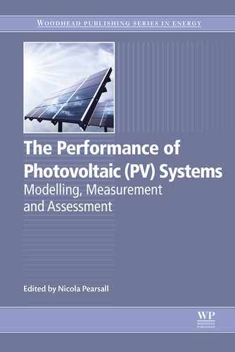
• The wind load is calculated based on the wind zone. In Switzerland, for example, seven wind zones are defined, with the levels of 0.9, 1.1 and 1.3 kN/m2 in the typical residential areas of Switzerland rising to 3.3 kN/m2 in the most exposed Alpine locations. In Germany, four wind zones are described, with up to three subcategories showing static pressure values between 0.5 and 1.4 kN/m2, the latter on small islands in the North Sea.
• Wind load increases roughly with the square of the height of the building. The resulting static wind pressure is given by a tabulated coefficient according to the height exposure category, which has to be multiplied by the preceding wind zone static pressure.
• A second wind coefficient has to be multiplied to account for the surroundings of the building. In Germany four zones are given: for a city, a village, flat country with trees and only flat country.
• The final wind exposure depends on the roof zone placement. For large roofs, the distance to the edge of the roof is relevant due to separation of strong vortices that then interact with the array's panel edges, especially for lightweight, low-slope, flat-roof PV systems. Again, relevant coefficients are given in the building codes to quantify these effects. Several manufacturers test their structures via experiments in wind tunnels and offer calculation methods and coefficients or web-based tools to address this complex issue (see Fig. 5.5).

• The total wind load is then split into the vertical load and the horizontal component which is relevant for the resistance-against-drag coefficient for movement of the whole structure.
• Snow load increases with the altitude of the location above sea level and depends on regional snow zone maps for each country. Recently, the Swiss SIA adapted their SIA 261:2014 snow codes for large flat roofs.
• The vertical load component has to be calculated from the overall wind and snow load together with the weight of the PV module itself. The values have to be well below the acceptable structural roof load of the building. On the other hand, a negative value, for example near the corner of a roof, may lead to lift-off damage of the PV modules. Thus the output of these static calculations may give different values of required ballast weight for different locations, for instance on flat roofs (see Fig. 5.5).
Polysun, a software tool to design and plan PV and solar thermal systems, at the time of this writing planned to offer as an additional feature a software-assisted calculation of the wind statics for several regions, including detailed suggestions for placing ballast elements, for example on a flat-roof PV installation [16].
5.2.2 New development and challenges of module mounting
Power losses and thermal hot spots may occur by unintentional growth of plants in between the rows of low-elevation PV mounting structures. To prevent these effects, the operation and maintenance cost will significantly rise or the costly insertion of an additional roof membrane will be needed (Fig. 5.6).

In some city centres, such as Chicago or Zurich, there are regulations to try to increase the number of green roofs to improve the ecosystem and incorporate water retention in case of heavy rains. In the future, more projects will arise to find synergies between green and PV roofs. Combining both the benefits of PV electricity production with green roofs, the need for higher PV mounting structures emerges, which will increase the costs relative to the common systems (see Fig. 5.7).

Other new approaches such as the mounting of bifacial modules [18] need a requisite amount of light collected by the backside of the PV module, which again leads to higher mounting structures compared to conventional low-cost, low-elevation systems such as are shown in Fig. 5.8. An interesting approach is to mount bifacial modules in a vertical position facing to EAST/WEST. This includes the benefit of making the gardener's task easier to perform, at reduced O&M costs. Another advantage of the bifacial approach is that the vertical PV modules do not generate the maximum power at noon compared to conventional south mounted PV modules (see blue curve in Fig. 5.8). Two production peaks, appearing in the morning (see red curve in Fig. 5.8) and the afternoon, lead to a better matching to the typical load profile. In future, the late afternoon load peak in particular will further increase due to the rising demand for charging of electrical vehicles. Thus costs for the daily peak shift of energy by the use of external batteries are reduced by the use of vertically mounted bifacial modules.

5.2.3 Orientation and yield of the fixed PV generator
Large MW parks or flat-roof systems are built as rows of PV modules oriented East/West and each module oriented south, with a typical inclination angle between 25 and 35 degrees in central Europe [20]. The design of the BOS component, the mounting structure, is relevant in regard to several percent of the final yield. The classical design rule assumes that shading starts to come from the PV module row in front towards south at noon in the wintertime, which results in a so-called shading angle of 20 degrees in central Europe [21].
Detailed measurement analyses performed in Zürich showed that, due to the foggy conditions in the morning and evening, standard commercial PV planning tools like PVSyst [22] overestimate the shading losses by up to a factor of 2. A grid with a mapping interval of 2.5 degrees for elevation and 5 degrees for azimuth is built and the amount of measured annual yield in each raster element is calculated (Fig. 5.9). Additionally, the shading limit (red curve) is drawn for a shading angle of 20 degrees in that reference test field.

The result of Fig. 5.9 was used to calculate a potential shading impact for each grid element. Consequently, the shading losses for different shading angles could be calculated using different models of how partial shading affects power losses. In the EKZ model A, the total yield is lost if the shadow hits the reference module. That means that partial shading has the same effect as full shading. This ends up with an overestimation of the losses. The EKZ model B delivers different yield losses depending on the sector where the shadow occurs. There are three sectors according to the bypass diodes. If the shadow line is located in the lower third, the losses are 1/3 of the yield. The losses are 2/3 in the middle third and 3/3 in the upper third. This loss classification into three areas is also used in model C. For shadow in the lower third, the losses are still 1/3. In all remaining cases, the yield is reduced to 10% assuming that 10% of the global irradiation is diffuse irradiation. This situation is more realistic due to the limited voltage range of each inverter.
Finally, these detailed loss analyses are compared in Fig. 5.10 with the findings of the commercial PVSyst software tool using different. There are large deviations of the shading losses with respect to the same angles. The losses for the standard shading angle used of 20 degrees vary between 1.5% and 4.9% and even 9% for another reference used (for further details see Ref. [23]).

Assuming shading losses of 2%, a shading angle of only 10 degrees is proposed by PVSYST while the detailed analyses based on real measurements as shown in Fig. 5.9 are based on a 20-degree shading angle. The latter offers an excessively higher total plant power output for the same standard flat-roof space.
5.2.4 Performance increase through mechanical tracking
Mechanical tracking of PV modules increases the electricity production of PV plants by about 20–30% relative to the annual yield of fixed installations, depending on location. Before the dramatic cost reduction of PV modules starting in 2009, from a level of about 3€/W to about 20% of that level today, several one-axis and two-axis tracking systems were developed and absorbed by the markets. At that time the additional costs of mechanical tracking systems relative to fixed mounting solutions increased the total plant costs by a percentage smaller than the increase of electricity yield due to tracking. This resulting economic benefit is reduced by the higher O&M costs associated with all the moving parts in the system (Fig. 5.11). Another reduction is needed due to the higher land requirement, because of the smaller capability of power extracting per square (compare Fig. 5.12).


A more theoretical approach showed that 41% more sunlight is available by mechanical tracking the PV module to follow the daily course of the sun, relative to fixed installations, if there is a very high amount of direct sunlight available, as in the most ‘suntrap’ locations on earth [24]. Calculated values between 31% and 36% of the two-axis gain in the Mediterranean region, compared to fixed installations, are achieved and predicted via public web calculation tools and also commercial PV planning tools [25]. Huld showed [26] that in Northwest and Central Europe, the relative gain of two-axis tracking is higher than in the south. In commercial PV plants, additional losses will occur relative to the single mechanical tracked module by shading losses of the nearby rows of also mechanically tracked PV modules on the limited available ground area of the plant. During the first three years of operation in Switzerland near Basel in a 650 kW PV plant, 23.5% gain due to one-axis tracking by solar wings with cable-based mounting solutions was measured [27]. Prototypes of such a cable-based tracker were installed in 2011 on top of a ski-lift in the Swiss Alps and on top of an outdoor storage facility in Flums in 2010, also in Switzerland (see Fig. 5.12).
At today's low PV system prices for large-scale fixed ground mounted plants, the 25% tracking increase in electricity yield will be covered mostly by the raw material stock exchange price of 200 kg steel needed per kWp to build the two-axis mechanical tracker [29]. New developments were performed optimizing one-axis systems to a very low demand of 100 kg/kW metal needed for the tracker. The mechanical PV tracker market accounted for only 3% of worldwide installed PV modules of about 1 GW in 2012 and about 4 GW were installed in 2014. In 2014 the world's largest single-axis tracking plant with a power of 206 MW started operation on an area of 801 ha on Mount Signal in southeastern California. Still, global annual installations of single-axis trackers are forecast to reach over 9 GW in 2019, driven mainly by the growth of utility-scale installations, as predicted by an IHS tracker market outlook [30].
Mechanical tracking still offers the benefit of increasing PV production in the morning and in the afternoon at a period when other south-mounted PV plants will not be able to supply the electricity grid in future (see Fig. 5.13). In the coming years, these extra costs of tracking may be economically more feasible than an electrical battery to close the gap between production of PV electricity and consumption.

New innovative concepts such as mounting PV modules on top of car parking areas and moving them in a safety box before very high wind or snow load occurs are only demonstrated at the prototype stage (Fig. 5.14). Such a solution will offer an extremely low amount of mounting material, but on the other hand might cause higher O&M costs.
Today most of the systems are still mounted on the rooftop with several centimetres distance behind the PV panel to the roof to benefit from better cooling compared to roof integrated PV systems. Besides the higher electrical performance due to the negative temperature coefficient of power, the O&M costs are much lower if PV modules have to be replaced, due to the much easier handling.
5.2.5 Reliability aspect of mounting solutions and O&M costs
The service lifetime of ground-mounted solutions is improved by choosing the appropriate material to avoid corrosion and designing the systems to withstand wind and snow load, which may be crucial depending on the location. Tracking systems will improve specific yield per installed nominal PV power but show a drawback in higher service time due to the moving parts in the plant. To limit the latter, only a small number of electrical drives per megawatt are used, equipped with dry bearing and a smaller tracking accuracy of 2% together with a robust mechanical design.
One of the single-axis tracker market leaders provides the power for parallel rows of 700 kW modules from a single lifetime sealed 2 kW AC motor including gearbox. The supplier is claiming zero-scheduled maintenance to the lifetime sealed drive and a mechanical system that features passive wind management that does not require active wind stow control or an uninterrupted power source (tested to 250 km/h wind, 3-second gust). This supplier published 99.996% uptime for their present products, responsible for tracking about 3 GW PV modules worldwide [32].
Industrial suppliers from India, for example, are installing seasonally adjusted trackers, which allow the angle of trackers to be changed seasonally by humans rather than with motors, at lower installation costs.
5.3 Electrical MPP tracking principles and losses
Maximum power (MP) production of the PV generator is reached by applying the appropriate DC voltage Vmp. Ten percent higher voltage than Vmp shows a loss of 16% of power, while 10% lower voltage than Vmp shows only 5% in power losses (Fig. 5.15). The topic of optimization of MPP tracking and related losses has been relevant in PV research and the PV industry for decades. The experimental findings are in accordance with the modelling output of the electrical current voltage characteristics of a solar cell, since the groundbreaking publication of Shockley in the middle of the last century [33] (see also Chapter 1).

In real operation, a deviation of the standard test conditions (STC) voltage given in the module datasheet occurs due to:
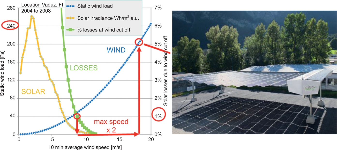
• Increasing solar irradiance Pin in the module plane will lead to a rise of Vmp as a function of the logarithm of the intensity (Vmp = c ln(Pin/P0) with c and P0 being constant factors) if the cell temperature is not changing; in detail it is not the power of irradiance that has a linear relationship to the short-circuit current but the number of photons with energies higher than the bandgap that are proportional—see Fig. 5.16.

• Increasing temperature T of the solar cell, the voltage Vmp will decrease by approximately 2 mV per K at constant current in standard crystalline silicon solar cells, as with silicon semiconductor diodes. The negative value of the temperature coefficient TCV leads to the smaller voltage Vmp(T) = Vmp_STC (1 + TCV (T − TSTC)) compared to the value at STC temperature of 25°)—see Fig. 5.16.
• Partial shading conditions on a crystalline silicon module equipped with typically three bypass diodes may show one absolute and one additional local maximum of power versus voltage. This number of total maxima may be equal to the number of bypass diodes depending also on the shading conditions—see Fig. 5.17 (cause of shading losses may be nearby objects like houses and plants or building elements, mountains, the next row of PV modules or soiling, starting from the PV module edges).

• Faulty conditions in either the module wiring of the cell interconnectors and/or the junction box shunting or broken wires will show a fundamentally different power output than expected STC power, mostly zero power.
• Degradation of individual solar cells will lead to problems, for example the decrease of the fill factor of an amorphous silicon solar cell due to light-induced degradation of up to 10% [36].
The optimum voltage to reach MP will be a mixture of the real outdoor or module conditions described previously. The results of the occurrence of Vmp values of a polycrystalline silicon module, without major failures or shading, for the summer half-year operated in Zurich, with measurement intervals of one minute, are shown in Fig. 5.16. At 1000 W/m2 irradiance, the Vmp in that practical application is 18% below STC value at a module temperature of 65°C. It is only 4% lower than Vmp_STC for the same irradiance at much lower ambient temperatures, leading to a final module temperature of only 35°C.
The measured real outdoor mapping for July 2015 of the MP operation conditions for voltage and power is given for the same reference installation for two different module technologies, polycrystalline silicon and heterojunction silicon, in Fig. 5.18. They use the same mounting conditions and have the same orientation. It is obvious that the voltage span at the same output power is much smaller for the heterojunction modules due to the smaller TCV value. A further small increase of that voltage span is found by comparing the string voltage for serial connection of the modules in Fig. 5.18. This is due to the real imperfect MP tracker performance of the commercial DC/AC inverter behind the string date compared to the mapping picture of a single reference Vmp calculated from each I–V scan of the single reference PV module mounted in the same installation.

Due to the fact that not all serial connected modules offer the same current at the individual MP, mismatch losses will expand the voltage span of the string shown in the voltage power mappings.
Even if a deterministic model is used, appropriate for the relevant module technology, and the cell and the cell temperature are measured together with the irradiance, this highly sophisticated MP voltage predictor will fail if partial shading (Fig. 5.17) or faulty wiring conditions occur by accident in such a module string.
5.3.1 MPP tracking algorithm and performance
Over the last few decades several methods and algorithms have been developed to operate PV generators at MP. A fast-changing irradiance at days with conditions that alternate between cloudy and sunny every few seconds or minutes (see Fig. 5.19) is very challenging. Improved algorithms are needed to handle emerging local power voltage maxima due to partial shading or faulty conditions in the module wiring (Fig. 5.17). Switching power electronic converters (see Section 5.4) are used to adapt the DC voltage on the PV generator, enabling it to track the new optimized MPP, forming a maximum power point tracker (MPPT).

The highest MPPT efficiency values are reached with clear-sky conditions at smooth solar irradiance characteristics compared to cloudy days (Fig. 5.19). The measurement uncertainty is typically much higher than 1% compared to the indoor laboratory measurements which could reach uncertainty values below 0.5% [39]. To achieve low uncertainty measurements under real outdoor conditions, longer averaging periods are helpful but also limiting for fast irradiance changes. The annual outdoor measurement of the inverter efficiency of a 650 kW PV plant in Waldshut, Germany was in accordance with the 97% euro efficiency given by the manufacturer of the 30 kW inverter [40].
MPPT algorithm—perturb and operate
The most widely used MPPT method is to increase the voltage of the PV generator Vmp to reach the new operation point at higher maximum power. The resultant power before and after that small period of seconds or minutes is measured. Depending on the sign of the voltage change and the sign of the power change, an optimized next small change of the voltage, a voltage step is proposed by the algorithm. Four different logical input states are possible and the resultant change of the next voltage presetting is defined by a simple logical diagram. This algorithm is called the perturb and operate (P&O) or hill climbing MPP method (Table 5.4).
Table 5.4
Logical rules/diagram according to the P&O MPP algorithm where V3 − V2 has an absolute constant value but changing sign and corresponds to the proposed new optimized voltage V3 which has to be applied to the PV generator as a result of the two measurements before the test period V1, P1 and during the test period V2, P2
| Process | V2 − V1 > 0 | P2 − P1 > 0 | V3 − V2 > 0 | |
| A | YES | YES | YES |  |
| B | YES | NO | NO | |
| C | NO | YES | NO | |
| D | NO | NO | YES |

Disadvantages of the P&O method are:
• Oscillating around a constant MP voltage at very constant irradiance conditions leads to losses during suboptimal operating conditions besides MPP (a smaller voltage step could then be used).
• If process A is performed with starting voltage V1 below MP and V2 as shown, then the next voltage step point is in the wrong direction (this is solved by control or estimate of the irradiance); a similar problem occurs for process C around the MPP.
• Staying in submaxima at partial shading condition (this problem is solved by switching to larger steps of voltage changes).
• With very quick irradiance changes because of fast-moving clouds, the MPP tracker takes too long to find the MPP.
The modified P&O method was proposed to solve some of these problems by decoupling the PV power fluctuations caused by the hill-climbing process from those caused by irradiance changes [41]. This method adds an irradiance-changing estimate process in every perturb process to measure the amount of power change caused by the change of irradiance condition, and then compensates for it in the following perturb process. There are two operation modes named: Mode 1 for an estimate process and Mode 2 for the perturb process. Mode 1 measures the power variation due to the previous voltage change and irradiance change, and keeps the PV voltage constant for the next control period. Mode 2 measures the power variation and determines the new PV voltage based on the present and the previous power variations. The tracking accuracy is significantly improved by this estimate-perturb-perturb (EPP) method. The perturb process conducts the search over the highly nonlinear PV characteristic, and the estimate process compensates the perturb process for irradiance changing conditions. Further improvements are reached by estimating the expected slower voltage decrease after a fast and strong irradiance increase.
MPPT algorithm—incremental conductance
A very efficient, robust and fast tracking method uses the ratio of current and voltage and the differential conductance near the MP of the PV generator characteristics. The differential conductance is calculated by the small current change resulting from a small increase of the voltage and is reciprocal to the differential resistance. Additionally the absolute conductance, the ratio of the absolute value of current and voltage have to be calculated. In a very rough method only the sign of the difference of the absolute and incremental conductance may be used, positive below Ump and negative above to control the PV generator voltage. It can be seen in Fig. 5.15 that the IV characteristic of a solar cell shows a smaller value of the differential conductance below Vmp compared to the absolute conductance. Only at the MPP does the difference between absolute and differential conductance diminish. The control strategy is to minimize the difference. This can be done using a constant period and constant voltage step as given in Table 5.5. This will result in an exponential convergence of the voltage to the optimum if the value of the step voltage is constant (see Fig. 5.20). Another advanced solution is to calculate the value of the voltage step as a function of the difference of both absolute and differential conductance values. Other faster and more efficient modified incremental conductance (IC) methods adapt the step voltage value depending on the difference of the absolute and incremental conductance.
Table 5.5
Principal of the IC MPPT algorithm based on the comparison of the absolute I/V and differential conductance ▵I/▵V of a solar cell characteristics near the MP voltage. Vmp2 is the resulting proposition of the PV generator voltage for the next voltage step with a step size of Vstep
| Sectors of the IV characteristic | Condition at Ump1: I/V > │▵I/▵V│ | Next voltage: Vmp2 = Vmp1 + ▵Vs |
| V < Vmp | Yes | ΔVs = + Vstep |
| V > Vmp | No | ΔVs = − Vstep |
Table 5.6
PV inverter power classes for AC grid operation and worldwide market share [44]
| Type of PV inverter | Power range | Efficiency | Market share |
| Central inverter | > 100 kW | < 98% | ≈ 57.5% |
| String inverter | < 100 kW | < 98.5% | ≈ 41% |
| Micro-inverter | < 400 W | ≈ 1.5% | |
| DC/DC optimizer | Module range | 98.8% without DC/AC | n.a. |

Table 5.7
Definition of key figures to describe the energy flow, typical on a yearly interval [77,78]
| Key figure abbr. | Key figure | Formula (see Fig. 5.24) | Description |
| PVG | PV grid | E1 | PV electricity feed into the public AC grid |
| PVS | PV stored | E4 | PV energy consumed via the battery storage |
| SCR | Self-consumption rate | (E4 + E5)/(E1 + E2 + E3) | Ratio of consumed PV energy to total PV production |
| ISCR | Immediate self-consumption rate | E5/(E1 + E2 + E3) | Ratio of immediate consumed PV energy to total PV production without storage “natural self-consumption” |
| SSR | Self-sufficiency ratio | (E4 + E5)/(E4 + E5 + E6) | Ratio of total load demand covered by the PV battery system |
| PSR | Prosumer ratio | (E1 + E2 + E3)/(E4 + E5 + E6) | Ratio of produced PV energy to total energy consumption |
| SCPVh | Storage capacity PV hours | C/Pn [kWh/kWp], [h] | Ratio of used nominal battery capacity to nominal PV STC power |

Before using a micro controller, hardware analogue solutions of the IC method suffered from the ripple of the measured current and voltage and thus unrealistic jumps of the incremental conductance occurred in real outdoor operation. Similar problems exhibit at fast changes of irradiance. Still today a high quality high bit analogue digital converter has to be implemented to provide low error IC tracking results.
MPPT algorithm—hybrids
More than six families of MPP tracking algorithms were reviewed by Onat [42]. The most powerful solutions in high-quality inverters are a combination of several methods implemented in the control software. To avoid, for example, being locked on a local maximum of the I–V curve, methods were developed to apply larger voltage steps in longer periods to test for the absolute maximum. In the IEC standards (see Section 5.5) procedures are defined to test the MPP tracking quality by defined ramps of irradiance for days with a fast change of cloudy and sunny conditions.
5.4 Basic power electronic concepts and losses
5.4.1 Basic principles and losses in power electronic circuits
The very first photograph advertising photovoltaic components shows a PV module by Bell Telephone Systems together with a lead acid battery and a smiling family back in the 1950s [43]. About 60 years later, innovative new products are coming onto the market offering to feed PV electricity into the grid and additionally offering the option to store electricity in so-called house storage batteries to use at night (see Section 5.5.2; Table 5.8).
Table 5.8
Simulation results of key figures according to Table 5.7 based on measured PV production data of a PV rooftop installation (Germany) [80] in 2012 (annual yield of 1131 kWh/kWp) and a measured typical single-family house in Switzerland with a consumption of 5511 kWh/a, performed at 15 min intervals. The simple cost estimates are calculated on 1300€/kWh installation costs including power electronics and an operating duration of 10 years for the battery system without financing costs or incentives. (Available rather than nominal kWh capacity values are used, with round-trip charging efficiency of 95%.) [81]
| PV sizing PSR | Battery sizing SCPVh (h) | Self PV consumption ISCR | From storage SCR-ISCR | Self-sufficiency SSR | Annual usage battery cycles | Costs storage €/kWh |
| 1 | 1 | 34.2% | 22.3% | 56.5% | 253 | 0.51 |
| 1 | 2 | 34.2% | 28.9% | 63.1% | 163 | 0.80 |
| 1 | 0.5 | 34.2% | 13.6% | 47.8% | 307 | 0.42 |
| 2 | 1 | 20.3% | 16.8% | 74.2% | 190 | 0.68 |
| 2 | 0.5 | 20.3% | 12.6% | 65.8% | 286 | 0.46 |
| 0.8 | 2 | 39.8% | 31.7% | 57.2% | 179 | 0.73 |
| 1.2 | 0.5 | 30.0% | 13.5% | 52.2% | 305 | 0.43 |
| 1 | 20 | 34.2% | 34.8% | 69.0% | 20 | 6.50 |

A resistive load directly connected to the PV generator always finds changing operating conditions and thus the value of the load resistor needs to change to extract the optimum power at maximum power point. Such simple circuits are very cheap because they only use one switch to disconnect the load. However, directly connected applications deliver losses due to not operating the PV generator at MPP all the time, such as directly charging a battery. In the last decades, widely used PV chargers with typically 36 serial-connected crystalline silicon solar cells per module were installed to power standard 12 V nominal lead acid battery sets. These 36-cell PV modules were chosen due to the voltage drop in this stand-alone PV battery system from the MPP to the maximum charging voltage of close to 14 V on the battery terminals. Today's standard 72-cell modules would be appropriate to power 24 V lead acid systems in a similar approach for very simple and robust PV DC storage systems (Table 5.6).
DC/DC converters solve this problem by decoupling the voltage level at the PV generator from the output voltage at the load. For decades, switched power electronic circuits were developed for up or down conversion for electrical drives, telecommunications and PV, decreasing the losses for the best products on the market from 8% in 1995 to about 1–2% today [45] (Fig. 5.21).

Typically the core of each switched circuit is to apply a different voltage level to an inductor, which carries the load current. A positive voltage for a short period of time is applied to the terminals of the inductor, leading to an increase in current followed by a small period with a negative voltage and a further decrease of the inductor current. By permanently adapting the length of the periods and the average value of the load current, the current of the PV generator is controlled. This method is called pulse-width modulation (PWM) and has been used since the beginning of semiconductor applications [46].
Different topologies are developed to place different semiconductor switches by means of appropriate DC voltage levels for the desired small period onto the inductor. This principle is also used in DC/AC inverters to directly connect the PV generator to the AC grid and thus control for a sinusoidal inductor current of 50 Hz (see Section 5.4.3).
5.4.2 Power electronic basics of grid-connected inverter
About 4600 PV inverter types have been offered on the international markets in the last few decades [47]. The lowest prices in 2014 showed the highly reliable central inverter at about 80€/kW and 110€/kW for the smaller string inverter used mainly for PV plants in buildings. Three phase string inverters account for one-third of the world market. The smaller micro-inverter, offered over the last two decades to directly connect a single PV module to the AC grid, has a very small market share, in the 1% range. Distributed DC/DC converters, coupling one or a few modules to track them at the optimum MPP, have gained a slight market share and are specially installed in buildings with a chance of partial shading conditions. Together with the DC/AC inverter, which groups several distributed DC/DC optimizers, the total efficiency is about 1–2% lower compared to a standard, highly efficient string inverter (Fig. 5.22).

Up to now, very little independent information about the reliability of these optimizers and their service life in real outdoor operation has been published. It is expected that the higher operation temperature of the electronic components used, such as the electrolytic capacitors mounted close to the PV module, will lead to a reduction of operation lifetime. There is a risk of significantly increasing O&M costs as a result.
A 1% increase in inverter efficiency improves the annual output of the PV plant by the same amount. Thus 1% higher total investment costs are allowable to reach the same levelized cost of electricity production. In that case, this higher efficiency inverter can achieve 10% higher prices per nominal power, due to the fact that the total cost share of the inverter is only 10% (see Fig. 5.1). These economic considerations have been the driver to improve PV inverter efficiency gradually from 90% in 1990 to 98% today.
In 2001 the average efficiency of a PV inverter smaller than 5 kW was 92% euro-efficiency (see Section 5.1) with a maximum efficiency of 96% for the transformer-less products, developed in the decade before [49]. These inverters offer the benefit of no galvanic coupling of the PV generator and the AC grid together with the disadvantage of about 3% higher losses in the transformer itself. Thus most of these transformer inverter systems were grounded at the minus pole of the PV generator, in accordance with the regulations in the United States at that time.
In May 2002 Heribert Schmidt applied for a patent [50] of his transformer-less HERIC topology, increasing the efficiency of the industrial products of the Sunway Company to 97% by using fewer components. Other related topologies such as the H5 from SMA followed, pushing the efficiency up to current values, slightly above 98% [51]. Twelve string inverters are in the 2014 top listing of a performance test survey with average European efficiency values between 97.5% and 98.5%, followed by another 117 products with tested efficiency values higher than 92% [52].
Transformer-less inverters with additional DC/DC converters also offer a large DC input voltage range, for example between 250 and 750 V. Some thin-film module products showed power degradation effects if the electrical potential of the generator dropped below earth potential. Thus some manufacturers of transformer-less PV inverters offered topologies equipped with an internal additional DC/DC converter to quarantee that the PV module was always above ground potential [53]. The downside of that approach is an approximately 2% lower inverter efficiency. In the last few years, the thin-film PV module manufacturers have improved their products and the latter type of inverter is not relevant on the market today.
However, string inverters offer new features to cut active power, for example, to 70% of nominal load if the grid operator requests that mode. Today this is, in most cases, the cheapest solution for a distribution grid operator facing voltage problems. As shown in Fig. 5.23, at a limitation of the AC power feed into the grid to 70% of nominal STC PV generator power, the annual losses are 4.4% for the location in Zürich, Switzerland.

The control of reactive power is another new feature of string inverters which has been implemented in the > 100 kW inverter for several years, starting in the German markets. This allows the distribution grid operator to stabilize the local grid voltage. The arising design challenges for inverter manufacturers are to increase the value of nominal electrical capacitors and handle the higher current.
These recently implemented functional features of PV inverters are able to handle the feed-in of a high amount of PV electricity into a distribution grid of, for example, a small village. Thus, in such cases about 50% of the electricity consumption could be delivered by the PV inverters without additional investment in expensive smart grid technical solutions [54].
A few inverter suppliers offer products on the market able to control a heat pump and the charging process of electrical vehicles using a weather algorithm at nearly no additional cost.
5.5 Results of BOS-related performance aspects
5.5.1 Performance of grid-connected PV systems
DC/AC inverter efficiency
The ratio of the DC input power reduced by the inverter losses and the DC input is called the conversion efficiency. Losses in power electronic devices may be separated into switching losses that are proportional to the inverter power P, resistive losses that are proportional to the square of the power and losses that are considered to be constant. Due to these different sources of losses and loss characteristics relative to the PV generator power and voltage, the inverter efficiency is not constant. The power of the sun changes during the day and thus the inverter efficiency depends on the individual share of the different loss mechanisms in the inverter. The measured losses of the PV inverter may be fitted to the following equation to get the relevant efficiency for a given power (see Fig. 5.24).


The resulting fitting parameters a0, a1 and a2 may be attributed to different loss mechanisms. The resistive losses are produced by semiconductor switches or inductors, the switching losses again by the power transistors and diodes and the constant losses come typically from the power supply and microcontroller or internal fan. Back in 1991, Hotopp proposed weighting factors to calculate the annual average inverter efficiency [56]
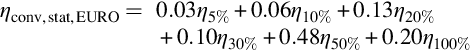
They are multiplied with the measured efficiency of the inverter under test in the laboratory at 5%, 10%, 20%, 30%, 50% and 100% of nominal power. The weighting factors were identified for the region of the Rhine valley in northern Germany, but have been established as a standard for the whole of Europe since then and are called the Euro efficiency value. Other weighting factors were proposed to have some additional values between 50% and 100% but the preceding coefficients are now established as the relevant norm [57] for testing inverters. The California Energy Commission (CEC) also defined weighting factors appropriate to the irradiance conditions at their locations:
These conversion efficiencies are measured in the laboratory at a static operation point of DC input and AC grid output and thus have the index ηconv,stat. Switching losses will increase with the DC voltage level. In the field the inverters are not operated just at a single DC voltage level, and thus ηconv,stat also has to be measured at several DC voltage levels within the MPP range. Hence, the coefficients of the power losses a0, a1 and a2 each must be enhanced by a polynomial term as a function of the DC voltage V:

Ten years ago only one value of the Euro efficiency was relevant on the PV market for most of the installers and planners. Knowledge about the real efficiency, which also varied up to 3% with the DC voltage, was missing for products on the market at that time. It was evident that 2% higher efficiency affects the inverter prices significantly. At about 20%, the share of the inverter is about one-tenth of the total costs. In 2004, this voltage dependency was published [58] and a year later the voltage mapping as shown in Fig. 5.23 was published at a specialist photovoltaic conference.
In the same year, Photon magazine published, in their annual PV inverter market survey, Fig. 5.24 together with other detailed technical data of 234 inverters on the German market [59]. Several requests followed from planners and installers to the suppliers of the inverters regarding the DC voltage chosen to calculate their Euro efficiency value given in the data sheet. Several suppliers started to present the Euro efficiency, for example, at three DC voltage levels. Photon magazine started to discuss the performance including the power voltage mapping of a single inverter per issue and offered further detailed data to the customers. In the published ranking list of inverter Euro efficiencies, the resolution is given as 0.1%. It should be taken into account that the measurement uncertainty of the efficiency in the laboratory is typically between 0.6% down to 0.2%, at a confidence level of 95%, for high-quality equipment and an experienced operator [60].
Today, the relevant norms propose efficiency measurements at different DC voltage levels. The voltage variations of that static conversion efficiency tend towards values below 1% due to the higher overall efficiency level.
The European Standard EN 50530 [61] provides a procedure for the measurement of overall efficiency of grid-connected photovoltaic inverters. It includes the definition of a procedure to measure the static conversion efficiency and also dynamic efficiency, describing the accuracy of the MPP tracking (MPPT) of inverters. Several publications discuss the approach to total efficiency as presented in the following [39,62,63].
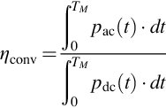
The overall efficiency ηt is defined as the ratio of the AC power output and the theoretical maximum available DC input power at MPP within a defined measuring period TM; this is also valid for changing MPP values of voltage and current:

The measurements of the final ηt are separated into the two categories of static conversion efficiency and dynamic MPPT efficiency:
The static conversion efficiency ηconv is measured as the ratio of the AC energy output to the DC energy input over a measurement period of 10 min. Measurements must be taken at 5%, 10%, 20%, 25%, 30%, 50%, 75% and 100% of nominal power at three voltage levels [63] (see Section 4.3.1 in Ref. [63]). There are more sampling points of power compared to the Euro efficiency weighting factors. But in an annex to the standards the previous old weighting factors are given and the resulting Euro and CEC efficiency values finally have to be calculated.
The MPPT efficiency ηMPPT is measured as the ratio of the energy drawn by the device under test to the energy provided theoretically by the PV simulator for operation at MPP.

where pmpp(t), pdc(t) and pac(t) are the instantaneous values, respectively.
The given selected input parameters and definitions are necessary.
Vdcmin/Vdcmax is the minimum/maximum input voltage; Vdc,r is the rated input voltage; Vmppmin/Vmppmax is the minimum/maximum MPP voltage; Idc,max is the maximum input current; Pdc,r; rated input power (or derived from AC power ![]() )
)
The requirements for the PV array simulator and the other test environment necessary for the measurements are defined in the standard. This includes tables of the required fill factor and voltage levels at MPP for the PV simulator distinguished between crystalline silicon and thin-film cell technologies.
To test the MPP tracker, ramp gradients ranging from 0.5 up to 100 W/m2/s are used for the tests with two different irradiance levels, from 100 to 500 W/m2 and from 300 to 1000 W/m2.
PV inverter and PV generator sizing
One of the first tasks in the PV plant design is to find the correct number of serial connected PV modules to fit with the MPP tracking voltage range of the inverter. If the temperature coefficient of the PV module is not taken into account and the nominal STC module voltage was used only to reach the lower inverter MPP voltage range, very high power losses will occur in summer (see Fig. 5.25). This will limit the lowest possible voltage of the MPP inverter tracking to an individual module voltage of about 15% higher than the optimum Vmp. As was discussed in Section 5.3 (see Fig. 5.15), this much higher operation voltage relative to Vmp will result in roughly 50% losses compared to MPP.

Another output of the mapping is the appearance of a constant voltage fixed tracking, as can be seen in Fig. 5.25 in the maxima at low power and 97% of STC string voltage in the right-hand plot.
Quality of MPP tracking
Especially at irradiance ramps of larger than 10 W/m2 per second, significant tracking losses are found [65]. Still today not all of the inverter manufacturers deliver products with robust MPP trackers, especially those suppliers who do not have many years of experience in the PV field (see Fig. 5.26).

The detailed test reports published by some technical photovoltaic magazines and performed in high-quality test laboratories provide an independent measured value of the Euro efficiency, which in most cases is in very good accordance with the manufacturer data sheets [66]. There is often helpful information as to whether there are problems regarding the practical quality of the MPP tracker, which otherwise a single user would be unable to detect. Again, in most of the reports, the MPPT efficiency is very high and overall efficiency is equal to the static conversion efficiency. But in some cases, these tests find faulty operating conditions. For example, an automatic disconnection from the grid was detected due to reducing the power factor from 1 to 0.7, and thus the resulting current value was above the shut-off limit [67].
Performance and wiring losses
A very common design approach is to limit the ohmic losses of the DC wiring to 1% when the PV generator is operated at STC power. Due to annual distribution of the produced DC power (see Fig. 5.23), the final ohmic losses over one year depends on the location and is roughly between one- or two-thirds higher than the ohmic losses at STC. To control this in real outdoor operation, mapping of the Vmp may help (Fig. 5.25).
5.5.2 Performance of grid-connected and storage PV systems
The very first advertising photograph of a photovoltaic module was presented as the ‘Bell Solar Battery’ together with a lead-acid battery by the Bell Labs back in 1954 [68]. Today this combination has become more important for improving the rate of self-consumption and unburdening the electrical distribution grid.
In Germany about 30,000 PV AC systems equipped with battery storage were in operation at the end of 2015, mainly in private households [69]. Thus, PV electricity could be applied via the battery even after sunset. About a 59% share of global storage installations were accounted for by the United States, Japan and South Korea in 2015 and 2016, and the UK will add 1 GW of storage facilities by 2020 [69]. Some of the storage market actors, claiming cost parity for large storage in 2015 in the UK, were supported by a feed-in tariff (FIT); others are expecting cost parity for smaller residential building solutions till 2017 [70]. A detailed survey of the German markets in 2015 based on 75 products resulted in storage costs of 5 kWh in the range of 0.3–0.7€/kWh and 0.2–0.6€/kWh for 10 kWh systems without subsidy [71].
These residential PV storage systems have been under intensive development during the last decade [72–75]. Reliable data on the performance of these grid-connected PV storage devices, as well as the quality of control, will be expected in the coming years, due to the fact that in Germany today half of the installed devices have been in operation for only one or two years.
Fig. 5.24 reflects the corresponding energy transfer which has to be controlled by the central power electronic conditioner. It includes the PV DC/AC inverter (see Sections 5.4.1, 5.4.2 and 5.3) as well as the battery charge controller.
To reduce this power electronics complexity, recently devices have been launched to operate only in the electricity exchange between the AC grid and the battery. This subsystem working in parallel with the PV system circuits is illustrated in Fig. 5.27 (see energy flow marked E7). Leading PV power electronic companies started the market introduction of such AC battery storage systems in 2016, heading for the potentially large retrofit markets represented by existing PV single-house system owners with numbers of roughly one million in each of the countries of Germany, the UK and Australia [76]. The installation costs of such retrofits are reduced and they are open for several battery products on the markets.
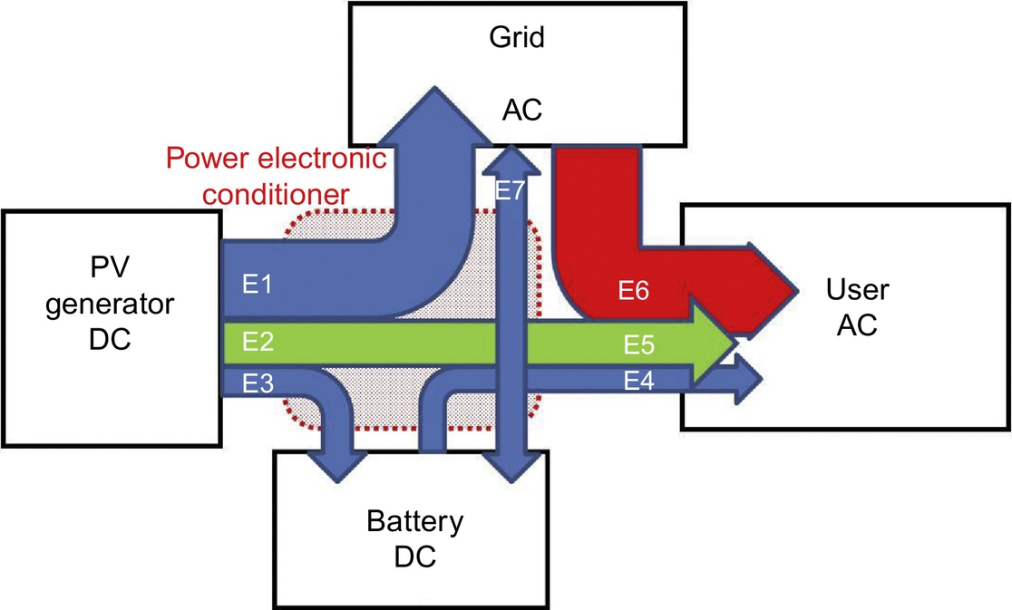
The definitions in Table 5.7 are widely used to describe the several energy flows shown in Fig. 5.24. The first one is the self-consumption rate (SCR), which specifies the share of PV electricity that is either used immediately or via the battery. Without the use of the battery the key figure is called the immediate self-consumption rate (ISCR) as given in Table 5.7. The self-sufficiency ratio (SSR) is given by the share of PV consumption to total demanded consumption. If the total amount of annual produced PV electricity equals the total consumption, the prosumer ratio (PR) becomes equal to 1. Even if PR becomes 1, electricity will be fed into the public grid due to the fact that the correlation between PV power generation and energy demand is not equal for each second during a year.
The annual electricity consumption in a single family house of 4500 kWh may be produced by a PV installation of about 4.5 kWp nominal power in most parts of Central Europe. Nevertheless, about two-thirds of the electricity consumption in the house is typically needed at periods with no PV production, for example in the evening. The real example in Fig. 5.28 shows a typical sunny day where nearly all the electricity consumed in the house was produced from PV and/or used after storing in the battery. On this day the self-consumption rate is 98%. Only in the early morning the battery is nearly empty and the needs of the coffee machine have to be powered by the public grid. This house is equipped with an 8 kWp PV system mounted on the rooftop and oriented to the west. The battery has a nominal power of 4.6 kWh (48 V lithium ion system).

It is obvious that doubling the PV power rating will improve the rate of self-consumption only marginally. The findings of several simulation runs of a standard residential load profile powered by different sizes of PV nominal power and battery capacity are given in Table 5.8. A simple PV battery charging algorithm was used. If PV production exceeds total consumption the difference was charged into the battery. The battery is discharged only to feed the load if PV production is too low.
Starting with a set-up to reach a prosumer ratio of PR = 1, about 56.5% (SSR) of the consumed electricity comes from PV at moderate storage costs of 0.51€/kWh. Thus 43.5% of PV electricity has to be fed into the public grid. By the use of the battery with a capacity to deliver the amount of nominal PV power for 1 h (SCPVh = 1 h), the immediate self-consumption of the PV production (of ISCR = 34.2% without a battery) is increased by 22.3%, to reach a total SCR of 56.5%.
Doubling the battery size increases SSR to 63.1% but also increases storage costs to 0.80€/kWh due to only 163 annual nominal capacity battery cycles during 10 years of operation. Doubling the PV power (PSR = 2) and reducing the battery size to only 0.5 kWh/kWp (SCPVh) leads to even a slightly higher SSR of 65.8% at very low storage costs of 0.46€/kWh. Thus, the PV self-consumption drops to SCR = 32.9%, increasing the cost of PV electricity production because two-thirds must be fed into the grid if the feed-in tariffs are low.
This example shows that, depending on the specific battery investment costs, battery cycles and battery lifetime have to be balanced with PV investment costs, the system's SCR and the feed-in tariff to reach an economic optimum at high SSR values. Today, with still relatively high specific storage costs, lower SCPVh design parameters are recommended.
Ref. [82] gives a detailed cost assessment for the German funding and feed-in regime results of a PV battery system on the limit of profitability to the 0.34€/kWh household electricity price for a system design with PSR = 1 and battery capacity of SCPVh = 0.6 h.
However, in the coming years, with higher cost reductions in storage compared to PV production, higher values of SCPVh and lower PSR values will be seen in the markets, and also a higher SSR will be reached. Additional loads like EV charging may change the key figures significantly.
Today PV battery markets are beginning to be developed and some of the first customers are premium option leaders where the costs are not the only issue to place their investments. Thus the battery capacity is designed to reach an SSR close to 1 during the summer period. This is illustrated in Fig. 5.29 by the simulated characteristics in one week in June of two PV battery systems, the second with twice the battery capacity.

Similar to the measured conditions given in Fig. 5.30, a daily simulation run performed (Table 5.8) results in about half of the capacity left in the battery in the early morning after that clear-sky day before. It should be mentioned that half the energy demand is at very low levels, below 0.15 kWh per 15 min interval, as is illustrated in the density plot of Fig. 5.31. Thus, it can be recommended that the most economical solution is first to reduce the load at night after midnight and later on to choose the appropriate battery capacity.


5.6 Reliability and durability
5.6.1 PV module reliability
During the 1970s, the terrestrial PV modules faced a lifetime of only 5 years. Significant advances were made to overcome the relevant failure mechanisms like encapsulant degradation and delamination and cell interconnection fatigue. In 1982 Mon and Ross at the Jet Propulsion Laboratory in Pasadena, California developed a systematic test approach in the form of an accelerated climate chamber test to speed up the development process to increase module lifetime to 20–30 years. For example, they proposed a thermal cycling between − 40°C and 90°C lasting only 430 cycles to exhibit the same fatigue effect to the copper-based interconnectors as for a real outdoor field exposure of 30 years at a much lower temperature difference of only 46°C, representing more than 10,000 real cycles [82].
Today, the same principles are applied worldwide during the crystalline silicon terrestrial photovoltaic (PV) module design qualification and type approval test, according to IEC 61215. Their test sequence 10.11 was established to determine the ability of the module to withstand thermal mismatch, fatigue and other stresses caused by repeated changes of temperature applied to two modules under test. This test lasts two and a half months by continuously cycling the temperature between − 40°C and + 85°C over a single period of 9 h, summing up to 200 cycles. The test is successfully passed if the degradation of maximum output power does not exceed 5% of the value measured before the test. These test sequences mainly verify the copper-based intercell connectors.
Upcoming new intercell connectors such as smart-wire technologies have shown much better reliability test results of power degradation below 5% even at 400 thermal cycles [83]. Further outdoor tests have to be applied before a higher operating lifetime of these types of PV modules may be concluded.
Additionally, another test, 10.13, is applied to two more modules of the same type, which are required to show a power degradation less than 5% after 1000 h of damp heat test at 85°C and 85% relative humidity. The focus of this test is the ability of the encapsulation of the module to withstand the effects of long-term penetration of humidity. To test the ability of the module to withstand the effects of high temperature and humidity followed by subzero temperatures, the humidity-freeze cycle was developed with 10 cycles with the same temperature as the 10.11 sequence, each having a period of 20 h at 85% relative humidity. Another mechanical test sequence, 10.16, determines the ability to withstand wind, snow, static or ice loads by applying 3 cycles of 2400 Pa uniform load, applied for 1 h to front and back surfaces in turn. This load corresponds to a wind pressure of 130 km h–1 with a safety factor of 3 for gusty winds (see Fig. 5.14). As an option for high snow load conditions, 5400 Pa static test conditions are applied during the last front cycle.
Thin-film modules have to pass another type of approval test, IEC 61646. With this, thermal cycling is not critical because thin-film modules typically do not use similar intercell connectors to standard crystalline cells. But other effects of light-induced degradation and UV testing are more relevant to failure mechanisms.
Some of the PV MW plant developers have set their own test sequences, using a strengthened climate chamber test. They simply increase the number of cycles for the 10.11 test sequence of the IEC 61215 and/or increase the duration of the damp heat test 10.13 by factors of two or four.
Long-term performance tests over 25 years at the European-Joint Research Center in Ispra confirmed that 82% of the 204 analysed modules have a final maximum power greater than 80% of the initial power and meet the manufacturer's warranty criteria [84]. Two-thirds of the modules showed output power values even higher than 90% of nominal power after 25 years in outdoor exposure.
5.6.2 Inverter reliability
Today's PV inverter products are typically offered with a standard 5-year warranty period with an extra charge of about one-third to expand the warranty to 15 years. In most of the operation and maintenance calculations the replacement of today's PV inverter is expected in 13 years, accounting for about 0.5% annual costs relative to the initial plant investment expenses [3].
In a survey performed in 2015 in the United States, the following vulnerabilities or reliability issues of PV inverters were found: electrical transient and grid events, dust and moisture, temperature cooling, components like fans, IGBTs, DC capacitors, boards, interconnects and loss of communication [85].
One critical component limiting the lifetime of the PV inverter is the aluminium electrolytic capacitor used in the decoupling of the AC current ripple of the PWM method from the PV generator. Due to evaporation of that electrolyte investigated in a 2000 h accelerated life test (ALT) at 105°C, the failure rate at lower operation temperatures is smaller by the acceleration factor AF, according to the well-known Arrhenius rule (AF(T) = exp[(Ea/kb)(1/Tref − 1/Tused)]) proportional to the ratio of failure rates with Ea the activation energy, kb the Boltzmann constant, T0 the absolute temperature in K of operation and T the accelerated testing temperature [86,87].
The thermic reaction speed is reduced and the evaporation of the electrolyte is roughly halved by reducing the temperature every 10°C. Several inverter manufacturers performed ALT at 50°C of the completed device for two calendar months permanently operated by solar simulators on the DC input [88].
Overvoltage may result in damage to the oxide film of the electrolytic capacitor, which then leads to a failure in the isolation layer and a loss of capacitance due to the anode foil as the dominant failure mechanism, decreasing capacity and increasing thermal losses [89].
To avoid this complex failure mechanism of the cost effective electrolyte capacitors, some manufactures have changed to the technology of foil capacitors, produced without electrolyte but at higher prices per capacity.
A few of the string inverter suppliers are using foil capacitors, such as Schneider Electric with their TL20000 E, and thus higher operating lifetime is expected but not explicitly stated in their advertising data sheets [90].
Some of the manufacturers assume a useful life of 10–15 years using electrolytic capacitors (mean time to failure (MTTF) = 2.7 million h) and 20–30 years for film capacitors (MTTF 2.6 million h) [91].
Concepts to assess the power electronics reliability of AC modules have been discussed, focusing on the same life cycle tests used for PV modules, according to IEC 61215, and damp heat tests at 85°C but for 2000 h [92]. Among the very scanty information about real tests of PV module inverters, TUEV reports of a still-working PV module inverter after 17 years of outdoor exposure in Arizona in the United States [93].
Only three inverters mounted on the back of the PV module have been tested, so that no statistically significant conclusion will be achieved. The type of inverter mounting solution is important, especially the air gap to the PV module back sheet, which is reported to be close to a maximum temperature of 95°C on this rooftop installation. The lack of information about the results of such reliability tests is expected to be replaced in the coming years by a broader techno-economic discussion driven by the increasing market share of microinverters and power conditioners.
5.7 Trends and Outlook in BOS
In 2009 the research group of ISE Freiburg exceeded the 99% maximum efficiency level by implementing a SiC power transistor in a laboratory scale PV inverter [94]. The remaining margin in improving Euro inverter efficiency on industrial products above 98–99% is limited by the costs of low-loss devices based on wide bandgap (WBG) semiconductors such as SiC or GaN. Reducing power losses also diminishes space, packaging material and thus the overall system costs of the inverter. Lower losses and lower maximum temperature of the critical power electronic components on the other side improves the service life of the system and thus the final generation costs of PV electricity.
In 2014 Google and the Institute of Electrical and Electronic Engineers (IEEE) launched the Little Box Challenge. It is an open competition with a US$1 million first prize to demonstrate a 2 kW DC/AC inverter and to shrink space down to less than the size of a small laptop (655 cm3) at a maximum surface temperature of the housing below 60°C [95].
Residential PV battery systems will follow a steady cost reduction as has happened in the last decades in PV module manufacturing, due to the industrial economy-of-scale effects. Starting from 0.35€/kWh storage costs in 2015 and assuming an annual cost reduction of 8%, it is expected that cost parity to the household grid cost, without energy, will be reached about 2025. This will only work for battery systems on the daily scale. The connection to the public grid will also remain with that connection cost, which will be oriented to the maximum of demand power and not to energy demand below a certain level. Later costs may diminish if the user disconnects from the public grid in a totally self-sufficient energy system, assuming an economic solution of seasonal storage.
The integration of the PV battery system into a residential system will be continuously improved by the most economical solutions such as controlling thermal loads via heat pumps or the charging of electrical vehicles, to reach the highest self-sufficiency ratios.
In these complex residential solar energy systems, reduction of the operation and maintenance (O&M) costs will be a key challenge in the coming years. It is expected that PV modules and inverters will not be the main O&M cost drivers compared to the batteries after 10 years of operation.
To fulfil these requirements, it is indispensable to implement design for reliability (DfR) in the development process of power electronics. In detail, attention must be paid to modularity and repair design, derating components, temperature management at reduced operating temperatures, different types of accelerated testing and applying predictive methods such as MTTF and DFMEA (design failure modes and effects analysis), fault tree assessments, and learning from reliability in allied fields, such as automotive and drives.