Photovoltaic module measurement and characterization in the laboratory
D. Dirnberger Fraunhofer Institute for Solar Energy Systems, Freiburg, Germany
Abstract
This chapter introduces basics of photovoltaic (PV) module measurement with regard to calibration and characterization. These tests play an important role for PV module manufacturers, purchasers and investors in PV projects, as they create important data on the quality of the PV modules under scrutiny, for example, in terms of conformity with data sheet indications or for prediction of PV system performance. Section 2.2 explains the underlying measurement process for I–V curve measurements and requirements for precise and accurate calibrations. The term calibration refers to standard testing conditions measurements performed by an accredited calibration laboratory. Section 2.3 gives information on the characterization, that is, the determination of other yield-relevant module characteristics. Section 2.4 adds some practical implications regarding module sampling, which is important for characterization of module types as opposed to characterization of individual PV modules.
Keywords
Module calibration; Module characterization; Measurement; Uncertainty; Thin film
2.1 Introduction
The output of a photovoltaic (PV) system depends essentially on the electrical performance of the PV modules in use, as outlined in Chapter 1. The ‘electrical performance’ of PV modules is described by different module characteristics that can be determined in the laboratory or outdoors. These module characteristics include electrical parameters at STC (standard testing conditions) as well as temperature coefficients (TCs), low light behaviour, spectral response (SR), angular response, thermal behaviour and module stability. STC are conditions that are widely used as reference conditions, and are represented by a temperature of 25°C and a broadband irradiance of 1000 W/m2 with a spectral distribution according to IEC 60904-3 [1].1
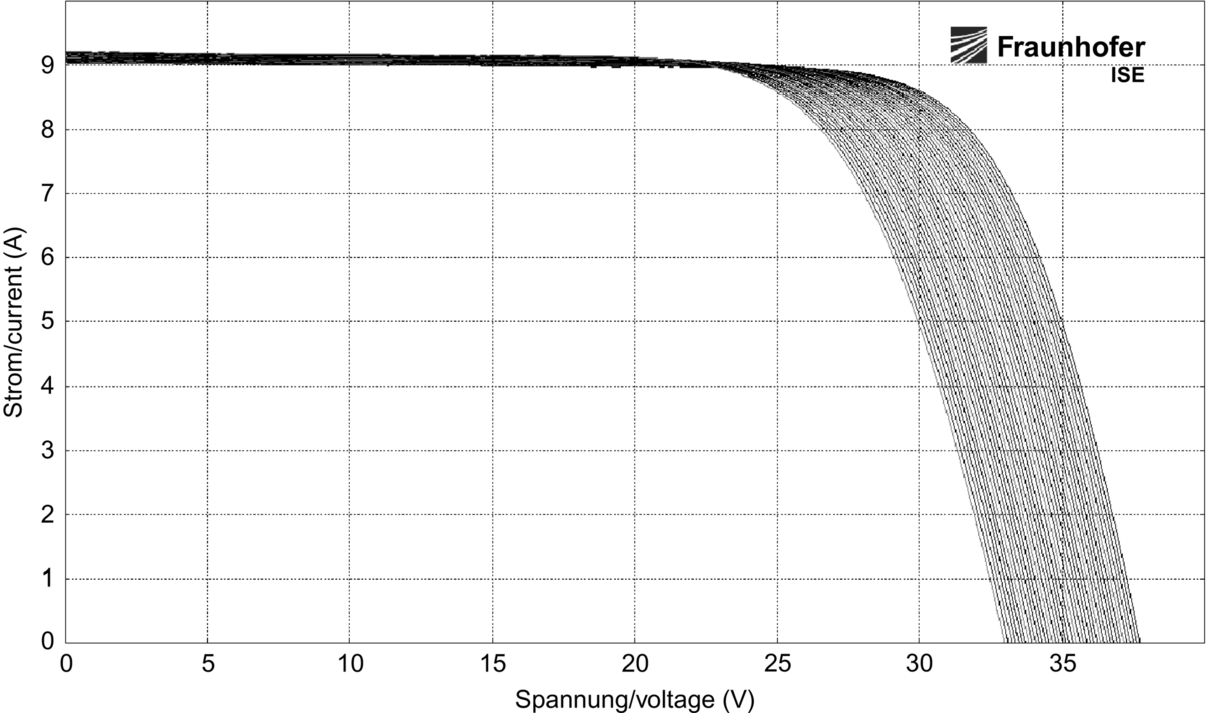
The ‘electrical parameters’ are specific points of the so-called I–V curve of the PV module. The electrical current and power created by a PV module2 under prevailing conditions depend on the voltage that is applied to the module terminals. The resulting current–voltage characteristic is shown exemplarily in Fig. 2.1, and is referred to as the I–V curve. Measurement of the I–V curve at defined conditions is the basis for determination of most of the previously mentioned module characteristics. The power–voltage characteristic, which is also shown in Fig. 2.1, is calculated by multiplying the current and the voltage values (P = VI). As it is inconvenient to report the whole I–V and its corresponding P–V curve, typically the following electrical parameters are presented as results: current at short circuit ISC, voltage at open circuit VOC, the maximum power PMPP, current IMPP and voltage VMPP in the point where power is maximal (maximum power point, MPP) and the fill factor (FF). These parameters are derived from the curves and, if necessary, used for further analysis (eg, TC, Section 2.3). The relevant equations for deriving the electrical parameters from an I–V curve and its corresponding P–V curve are given in the following:
where ISC is the short circuit current, which is the current when the voltage at the device terminals is zero.
where VOC is the open circuit voltage, which is the voltage when no current is produced.
where PMPP is the power in MPP. It is the maximum power the module can produce under prevailing conditions, and is usually determined by applying a fifth-order polynomial fit to the measured P–V curve around the expected PMPP.
where VMPP is the voltage in the MPP, which is the voltage that occurs where the power is maximal, that is, where the derivation of power with respect to voltage is zero.
where IMPP is the current in MPP.

where FF is the fill factor. FF basically indicates the magnitude of losses in the semiconductor structure [2].

The power conversion in a PV module and thus the values of the electrical parameters depend on module temperature and available irradiance (see also Chapter 5). Thus, the electrical parameters determined by measurement are influenced by the conditions during the I–V curve measurement. In order to achieve comparability of reported PV module parameters, the community agreed on the previously mentioned STC. As a consequence, PV module measurements involve not only measurements of electrical current and voltage, but also of module temperature and irradiance. For precise measurements of STC parameters, controlling the conditions during measurement (temperature, broadband irradiance and spectral distribution) and achieving only small deviations from STC is very important. Today, solar simulators are optimized for measurements at STC as a consequence of the key role of these conditions in the PV industry.3
Measurements at STC are also referred to as calibration or STC power rating of PV modules. The term module calibration can be used if the measurement is performed by an accredited calibration laboratory. The calibrated module is then used as a reference device for further measurements by testing or inhouse laboratories, or in a module production line for calibration of the simulator. The term STC power rating in this context designates the process of assigning an STC power value to a newly produced module and binning modules to STC power classes.
While modules can be characterized both by indoor and outdoor measurements, this section focuses on indoor (laboratory) measurements. The advantage compared to outdoor measurements is that the measurement conditions are much more reproducible and independent of current weather conditions or local climates. The role of PV outdoor performance assessments is explained in Chapter 3. Laboratory measurements are applied for several different purposes in practice. It is helpful for further understanding to be aware of the following purposes:
• Module development: Measurements of different module characteristics are performed in order to track the outcome of optimizations of module design and/or to document new record values. These measurements are carried out by inhouse or service laboratories and, mainly for external verification, by accredited laboratories.
• Module production: At the end of the production, each module is measured in order to assign the correct rated power (or STC power bin) to the module on its label. Calibrated reference modules are required for accurately setting the measurement parameters.
• Quality assurance: Out of a batch of purchased modules, a sample is measured in an independent laboratory to check data sheet specifications regarding STC power and other module characteristics. The acquired data can be used for performance prediction.
The following sections give more detailed explanation regarding the topics that were hinted at in this introduction. I–V curve measurements at STC and measurement uncertainty evaluation are discussed in detail in Section 2.2. This serves as a basis for the explanation of measurement of other module characteristics in Section 2.3. Section 2.4 briefly discusses aspects regarding variability of module characteristics and sampling of modules from batches for the purpose of quality assurance. Section 2.5 gives a short outlook on future perspectives.
2.2 PV module STC measurements using solar simulators
2.2.1 Measurement set-up and procedure
The typical set-up for laboratory I–V curve measurements is shown in Fig. 2.2. The set-up consists of:

• a reference device for determination of (broadband) irradiance during the measurement
• a structure to mount the device under test (DUT)4
• temperature sensors (Pt100, Pt1000, thermocouples or sometimes infrared sensors)
• an electric load to apply a changing voltage (voltage ramp) to the DUT while it is illuminated
• measurement instruments to record
○ the I–V curve (ie, the current the module produces at the applied voltage levels under illumination)
○ the temperature
○ the irradiance signal (ie, voltage or current of reference device)
Modern measurement systems also include software solutions for treatment of the measured data, most of all the correction to STC and determination of I–V curve parameters.
In the following, the measurement procedure will be described with a focus on secondary module calibration. Secondary calibration is calibration using a primary-calibrated reference device and creating a secondary reference device (Section 2.2.10). Details can be different for other measurement procedures depending on their purpose. The state-of-the-art rules for performing I–V curve measurements are also given in the IEC 60904-1 [3].
Prior to the measurement, the DUT is mounted so that a perpendicular line can be set-up between light source and module plane. DUT and reference device must have exactly the same distance from the light source. The temperature sensors are placed in a way that allows for correct measurement results (ie, Pt100 sensors are attached to the back of the DUT, infrared sensors must be properly placed and calibrated). The cables of the PV device (positive and negative terminal) are connected to a four-wire measurement set-up and electrical load. When the measurement is started, the electrical load applies a defined voltage sweep to the module while it is illuminated. The voltage at the device terminals and the resulting device current are measured. If a pulsed solar simulator (Section 2.2.2) is used, the electronic load must be triggered by the light pulse. After the measurement, the measured data must be treated, for example, smoothed, interpolated to standard voltage steps, and corrected to STC. Finally, the previously mentioned electrical parameters are derived and reported. The final measurement result should be the average of several measurements.
2.2.2 Characteristics and characterization of solar simulators
Different types of solar simulators are available. The main differentiation is between pulsed and continuous solar simulators. Pulsed solar simulators work with electric arc lamps (eg, Xenon arc lamps) that create a light pulse with a duration of much less than 1 s, while continuous solar simulators use lamps that provide constant light for many hours.
Typically, the manufacturers of PV measurement systems offer complete systems including the light source (solar simulator), a control unit for the light source and the measurement electronics (electrical load and measurement equipment). The characteristics and performance of the measurement system are essential for the achievable measurement uncertainty. While the quality of the measurement electronics affects the quality of the I–V curve measurement (Section 2.2.3), the quality of the light source affects the uncertainty of the irradiance measurement (Section 2.2.4). The most important characteristics of the light source are:
• Spectral distribution: the closer the match to the reference spectral distribution, the smaller are spectral mismatch errors even for different SRs of reference device and DUT (compare Fig. 2.5). The spectral distribution depends first on the type of lamp and second on filters that can be installed in between lamp and DUT.
• Nonuniformity: the better the uniformity, the smaller are errors due to misplacement of the reference cell, which should be placed in a spot with irradiance equal to the average irradiance available over the area of the module. Furthermore, good nonuniformity minimizes influences on the I–V curve due to cell currents that are mismatched because different cells receive more or less irradiance depending on their position.
• Stability of the light characteristics: stability of irradiance and spectrum during the measurement (ie, typically in an order of magnitude of 10–1000 ms) is essential, but also longer term stability is desirable as this facilitates measurement procedures. For example, it was observed at Fraunhofer ISE that the spectral distribution red-shifts with increased number of flashes, and also nonuniformity can change during the lifetime of the lamps used.
• Directional distribution of the light: The PV module is mounted so that a perpendicular line can be set-up between light source and module plane. In the ideal case, all the light is incident on the module plane perpendicularly. In reality, there is usually a specific aperture angle of the light source and optics, which causes widening of the light beam and leads to a specific distribution of angles of incidence on the module plane. Furthermore, there is a certain amount of stray light due to reflections of the surroundings, even though in high-quality simulators this is minimized as far as possible (eg, by using aperture masks).
• For pulsed solar simulators, an important feature is the pulse length. The pulse length determines the maximum measurement time for one I–V curve sweep, unless special methods such as section measurements are applied (see Section 2.2.3). Available pulse lengths are 10 ms to around 300 ms; long pulse simulators offer pulse lengths of up to around 800 ms.
The first three of the mentioned characteristics are used in the standard IEC 60904-9 for classification of solar simulators [4]. The directional distribution of the light is mentioned here for the sake of completeness. Looking at a solar simulator as a point source of light is a common approach, but only valid for very basic considerations. It is very difficult to accurately determine the directional distribution of a solar simulator, but fortunately this has not presented severe consequences for standard measurements in the past. However, measurement results can be influenced if DUT and reference device have significantly different reflection characteristics (Section 2.3.6).
Following the IEC 60904-9, simulators are attributed to a class for each of the first three of the mentioned characteristics, leading to classifications like ‘AAA’ or ‘ABA’. The criteria for the classification are summarized in Table 2.1. Following is a brief discussion of how the characteristics can be determined.
Table 2.1
Solar simulator classification according to IEC 60904-9
| Class | Spectral match | Spatial nonuniformity (%) | Temporal instability (STIa/LTIb) (%) |
| A | 0.75–1.25 | 2 | 0.5/2 |
| B | 0.6–1.4 | 5 | 2/5 |
| C | 0.4–2.0 | 10 | 5/10 |

From IEC 60904-9 Ed. 2.0, Photovoltaic Devices—Part 9: Solar Simulator Performance Requirements, International Electrotechnical Commission (IEC), Geneva, Switzerland, 2007.
a STI—short-term instability, the observed variation of irradiance from one measurement point to the next during one I–V curve measurement.
b LTI—long-term instability, the observed variation (max/min) of irradiance during one I–V curve measurement.
Measurement of the spectral distribution of a solar simulator can be quite complicated, especially in the case of a pulsed solar simulator. In this case, spectroradiometers with very short integration time and sophisticated equipment for correctly timing the measurement must be used. More details on the challenges can be found in Refs. [5,6]. The question of whether the spectrum changes during the pulse can be answered by repeating the measurement several times within one flash, which further increases the integration speed requirement. For accurate measurement results, the spectroradiometer must be well-calibrated, even though relative calibration is sufficient. Relative calibration means that the spectral distribution is measured in counts, which gives information only about the relative irradiance at a specific wavelength (eg, 60% compared to the wavelength with maximum irradiance) but not about the absolute irradiance in W/nm or W/m2 nm. Further information on spectroradiometer calibration and spectroradiometry in general can be found in Ref. [7].
The ‘spectral match’ according to IEC 60904-9 is determined with respect to the wavelength range from 400 to 1100 nm. For six defined wavelength intervals (100 nm step width except for 900–1100 nm), the percentage of irradiance within the interval compared to the total irradiance is calculated and compared to the corresponding percentage for the reference spectrum. The spectral match is the ratio of the percentage for the simulator and the reference spectrum:

where a and b are the limits of the wavelength interval under consideration, E(λ) is the spectral distribution as measured for the simulator and for the reference, respectively.
The classification of the simulator is equal to the worst classification of all intervals. As the spectral distribution of solar simulators has improved considerably in the past years, additional classifications like ‘A+’ (indicating a spectral match between 0.88 and 1.12) have appeared. While this is useful to better differentiate simulators with class A spectral classification in a general way, it has to be kept in mind that the significance of the classification in terms of measurement uncertainty is limited: the wavelength range under consideration is smaller than the SR of most PV modules, and the calculation procedure allows that deviations in opposite directions within one wavelength interval cancel out. Such deviations do not necessarily cancel out in the spectral mismatch calculation (Section 2.2.4), so that high uncertainties in spectral mismatch calculation can remain despite A + classification.
The measurement of spatial nonuniformity can be performed in two ways. In the first option, the area under consideration is scanned by one measurement device (eg, a calibrated industrial PV 15.6 × 15.6 cm2 cell or a reference cell with area of 2 × 2 cm2) that is moved from one position to the next. This method requires a rigid structure for exact positioning of the reference device and an additional reference device that is positioned in one constant spot throughout all measurements to check on the irradiance level at the time of each measurement. The second option is to build special measurement instruments that are comprised of several cells enabling the simultaneous measurement of irradiance in several spots (eg, the nonuniformity module used at Fraunhofer ISE as described in Ref. [8]). For both methods, the result is a matrix of irradiance values and the nonuniformity equals the difference between minimum and maximum irradiance, divided by the sum of these values. Fig. 2.3 shows example results for two different solar simulators.

The determined nonuniformity value depends on the size of the device used for the determination, the coverage of the whole area of interest with measurement spots (ie, how large the space is between measurement points), and the magnitude of the area of interest (module area). Therefore, comparability of nonuniformity values is limited. At least, the considered area should be stated along with the nonuniformity value—while 1% for 2 m × 1 m is a rather typical value, it would be a very good result for 3 m × 3 m. The measurement uncertainty of the determined nonuniformity depends a lot on the measurement procedure and, especially for the second method, on the calibration of the nonuniformity device.
The temporal instability can be measured with basically any PV device that is stable during the measurement. The determined value can be influenced by the sampling rate. Compared to the spectrum and the spatial nonuniformity, temporal instability is typically not an issue. Furthermore, the influence of temporal instability can be corrected after the measurement (point-by-point correction of the I–V curve; see Section 2.2.6).
2.2.3 I–V curve measurement
The conditions during an I–V curve measurement usually differ a little from STC, even though they are controlled. Therefore, the result of an I–V curve measurement always depends on the prevailing conditions, but this can be corrected before reporting the final STC result, as long as the I–V curve itself was measured correctly. This section on I–V curve measurement refers to aspects related to the measurement of the I–V curve itself, disregarding the conditions (but assuming small deviations from STC).
As mentioned previously, the positive and negative terminals of the DUT are connected to a four-wire measurement set-up and an electrical load. Four-wire measurement is essential for correctly recording both current and voltage—additional resistance in the connection before the four-wire measurement point creates a voltage drop which introduces a current-dependent error in the measured voltage:
where Vapplied is the voltage as applied to the module (and measured), VPV is the actual voltage at the PV device terminals, and R is the series resistance causing the error (Fig. 2.4).
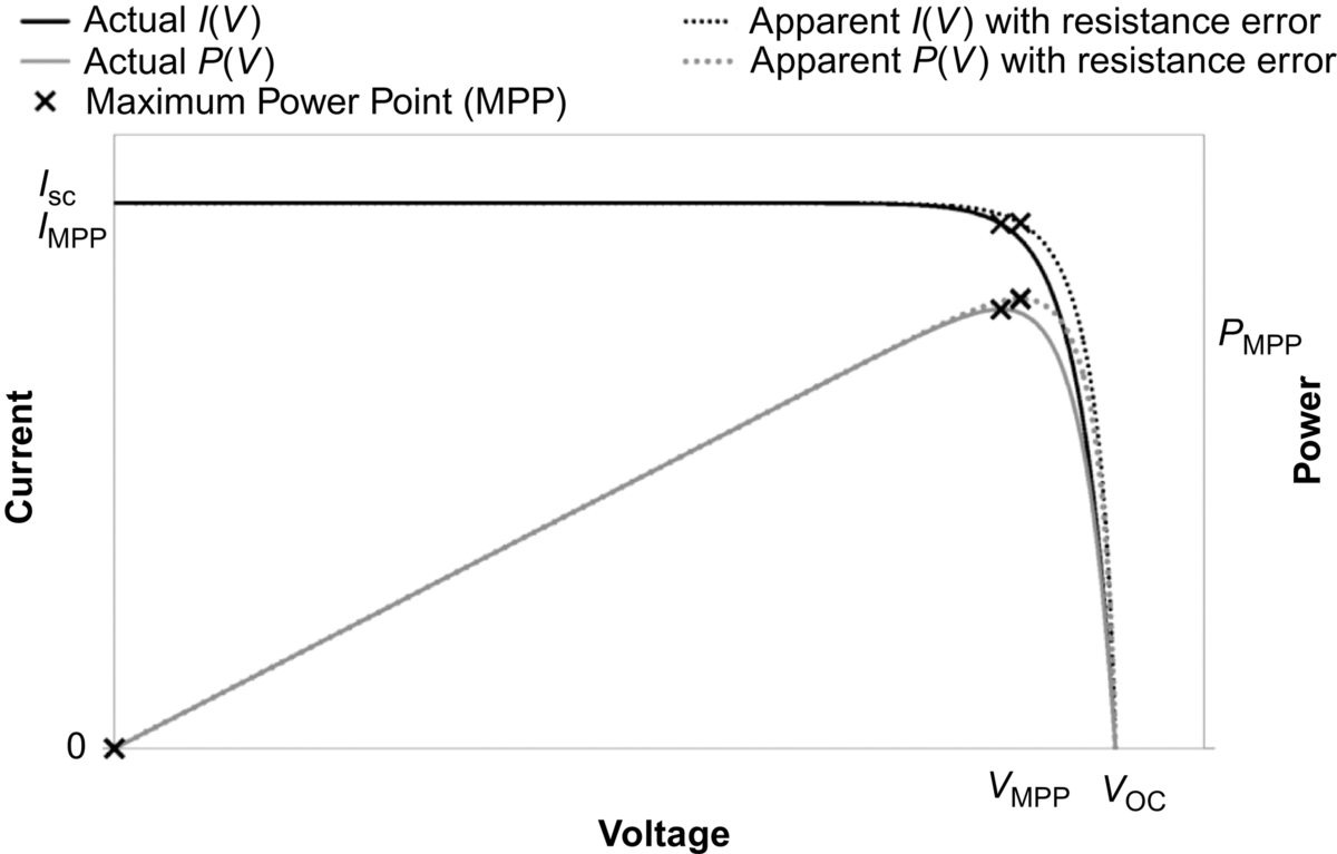
Such errors affect above all PMPP and FF. The four-wire measurement point for a PV module is typically the module plugs. For other PV devices, for example, with just busbars coming out of the mini module or encapsulated cell, one should report in detail how the DUT was electrically connected to avoid differences in measurements that cannot be explained.
After plugging DUT and measurement equipment, the I–V curve measurement can be started. The I–V curve measurement is essentially applying a voltage sweep to the DUT and in parallel measuring voltage and current of the module under illumination. For continuous solar simulators, the measurement can be started manually. When a pulsed solar simulator is used, it must be triggered by the light pulse. The electronics must be capable of measuring with a sufficiently high sampling rate, as the pulse length is often in the order of magnitude of only 10 ms. Prior to starting the measurement, the sweep profile of the electronic load must be defined considering the module characteristics and the available features of the measurement equipment. Finding the optimal parameters is usually an iterative process.
If a three-quadrant load5 is available, typically the voltage ramp starts a little below 0 V in order to overcome ohmic resistances in the cables, and to obtain a clear intersection with the y-axis (0 V; this is important for accurate determination of ISC). Similarly, it ends at a value somewhat larger than open circuit voltage to obtain a clear intersection with the x-axis (0 A). The sweep speed and direction play an important role. The sweep speed is the total voltage difference divided by the time, for example, 48 V/8 ms = 6 V/ms. Each solar cell and thus each PV module has a specific capacitance [9, p. 67], which causes a specific dependence of the current on the applied voltage and the direction of the voltage sweep. For ‘forward measurements’ (load voltage is increased from 0 V to open circuit), one can think of a capacitor within the module which is charged with the current, so that the power in MPP can appear smaller than the actual power. For ‘backward measurements’ (load voltage is decreased from open circuit to 0 V), this capacitor is discharged and adds current, so that the power in MPP can appear larger. The actual amount of over- or underestimation of PMPP depends on the combination of module characteristics and sweep speed.
To prevent measurement errors due to the described hysteresis effect, different methods can be used. Hysteresis measurements consist of one forward and one backward measurement. The difference between both measurements indicates the severity of the capacity effect. If the detected hysteresis ![]() is too large, it can be decreased by splitting up the I–V curve in several sections (ie, measuring parts of the I–V curve with several light pulses). This decreases the sweep speed and thus the hysteresis. A reasonable range is 0.5–1%. Alternatively, important points of the I–V curve can be measured using a ‘multiflash’ procedure, where the voltage is kept constant during the light pulse. The desired voltage level is set per pulse. Further special methods to deal with capacitive effects exist, such as the Pasan-developed Dragon Back method [10] or an algorithm developed by Halm for temperature dependence or power rating measurements [11] (compare also Section 2.3).
is too large, it can be decreased by splitting up the I–V curve in several sections (ie, measuring parts of the I–V curve with several light pulses). This decreases the sweep speed and thus the hysteresis. A reasonable range is 0.5–1%. Alternatively, important points of the I–V curve can be measured using a ‘multiflash’ procedure, where the voltage is kept constant during the light pulse. The desired voltage level is set per pulse. Further special methods to deal with capacitive effects exist, such as the Pasan-developed Dragon Back method [10] or an algorithm developed by Halm for temperature dependence or power rating measurements [11] (compare also Section 2.3).
2.2.4 Measurement of irradiance
The irradiance is measured using a reference device. Generally, the reference device can be smaller or larger than the DUT, or can have the same size. For secondary calibrations, the reference device is typically a primary-calibrated reference cell in WPVS (World Photovoltaic Scale) design [12]. For measurements in production, the reference device is typically a PV module of the same module type, ie, same kind and same number of cells compared to the produced modules.
In general, the irradiance indicated by the reference device is calculated using the calibration value and the measured signal:
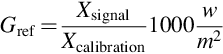
where Gref is the irradiance as measured by the reference device, Xsignal the signal (short circuit current, or the corresponding voltage measured via a resistance) of the reference device, and Xcalibration the calibration values, that is, the signal of the reference device at STC.
The calibration value of the reference device is one of the most important parameters affecting the measurement result. Therefore, it is essential that a reference device calibrated by an experienced and accredited institution is used.
The irradiance measured by the reference device can differ from the irradiance that effectively contributes to current generation in the DUT (‘effective irradiance’, [13]) mainly for the following reasons (compare Section 2.2.2):
• Spectral effects, quantified using the spectral mismatch factor (MM)
• Spatial effects, depending on nonuniformity
• Reflection/stray light effects
Theoretically, the effective irradiance can be calculated using correction factors as follows:
where G is the effective irradiance available to the DUT, Gref the irradiance as indicated by the reference device, MM the spectral MM for correction of spectral mismatch, Fnonuniformity a correction factor for nonuniformity errors in case the reference cell cannot be positioned correctly (see the following), and Freflection a correction factor for reflection-related errors.
The correction factors are strongly linked to the quality of the simulator light in terms of spectral irradiance, spatial nonuniformity and the directional distribution of the light as was discussed in Section 2.2.2. Including the MM quantitatively in measurements can be considered as state-of-the-art. The spatial nonuniformity factor is usually taken into account by positioning the reference cell correctly, that is, in a spot with irradiance equal to the average irradiance over the module area. The reflection factor is rather a wildcard character to illustrate here that such effects exist, but is typically not included quantitatively in measurements.
The spectral mismatch refers to the fact that PV modules have individual SRs, which means the conversion efficiency of light to current depends on the wavelength of the light. This causes the irradiance effectively contributing to current generation to be different for the reference device and the DUT—even at a spectral distribution equal to the reference spectral distribution. Fig. 2.5 depicts the spectral distribution of a c-Si and a CdTe module and a c-Si reference cell and demonstrates that differences in the SRs can be considerable. Furthermore, the spectral distribution of simulators differs from the reference spectral distribution (Fig. 2.5), which causes additional differences. The overall difference in the effective irradiance (ie, the irradiance that contributes to current generation in the DUT) is quantified using the spectral MM, which is calculated as follows:

where SRDUT(λ) and SRref(λ) are the (relative) SR of the PV DUT and the reference device, respectively, Emeas(λ) is the measured (relative) spectral irradiance under actual conditions and Eref(λ) is the reference spectral irradiance according to IEC 60904-3 [1]. The wavelength limits a and b should span the full range of spectral sensitivity of the DUT and the reference device. The transformation of Eq. (2.11) shows that MM can be written as a ratio of short circuit current values. This indicates that MM is the ratio of the effective irradiance difference between DUT and reference device at simulator spectrum, and the corresponding difference at reference spectrum.

The spectral MM can be used either to set the correct irradiance during the measurement or to correct the results afterwards. In the first case, the calibration value of the reference device is divided by MM, so that the indication of irradiance by the reference device during measurement already represents the effective irradiance for the DUT. A MM value larger than unity basically indicates that, effectively, the DUT can use a larger part of the incident irradiance than the reference device, that is, 1000 W/m2 effective irradiance is reached at a slightly smaller power level of the lamp. If the MM correction is performed after the measurement, this is technically synonymous to corrections to STC for cases where the irradiance level during the measurement was set too low or high (Section 2.2.6). A useful approximation is to divide ISC or PMPP by MM.
Spatial nonuniformity can cause offsets in measured irradiance, if the reference cell is placed in a spot that is particularly dark or bright (compare Fig. 2.3). The offset should be minimized by placing the reference cell in a spot with irradiance equal to the average irradiance in the module plane (see IEC 60904-1, Sections 6 and 7 [3]), but could also be corrected by a nonuniformity factor after the measurement. It can be difficult to find a generic location for the reference cell for arbitrary module sizes.
Apart from the discussed influences, the characteristics of the reference device are essential for correct measurement of irradiance. Most important is long-term stability, meaning that the calibration value (but also other characteristics such as SR or reflection behaviour) must be constant over a period of several years. Furthermore, linearity is important (compare IEC 60904-10 [14]), and the reference device should have a high FF in order to limit influences if a shunt resistance is used.6
2.2.5 Measurement of module temperature
The module temperature is usually measured by attaching temperature sensors (Pt100, Pt1000 or thermocouples) to the back of the module. Sometimes, infrared sensors are used. The ‘module temperature’ is the average of the indication of all sensors. Typically, laboratories set-up limits for deviation from the target temperature and limits for the deviation of individual sensors from the average. To ensure module temperatures close to 25°C, the laboratory and the area where modules are stored prior to the measurement have to be carefully temperature controlled. This helps to limit uncertainties due to two frequently discussed issues with module temperature determination:
• Is the temperature of the backside equal to the temperature of the cell and the p–n junction?
• Is the spatial nonuniformity of temperature within the module sufficiently small?
For measurements with pulsed solar simulators, this question is not crucial if good air conditioning is available, but is harder to handle for STC measurements using continuous solar simulators or natural sunlight. It is a really difficult question for continuous outdoor monitoring. In a production line, where the air temperature (and thus module temperature) cannot be controlled as tightly as in a laboratory, these two issues lead to a larger variation of module temperature and cause larger associated measurement uncertainty.
2.2.6 The correction of I–V curves to STC
The STC parameters are obtained by combining measured I–V curve, measured module temperature and irradiance. Even if measurements are made at conditions very close to STC, small deviations of 5–10 W/m2 or 1°C typically occur. These should be corrected to achieve best possible repeatability and comparability of results. Otherwise results from repeated measurements in one laboratory, or measurements from different laboratories, will differ from each other only because conditions were not identical.
Missing correction regarding irradiance mainly affects current (ie, ISC, IMPP and PMPP). The influence is linear, that is, a deviation of 10 W/m2 at 1000 W/m2 leads to a difference of 1% in reported current values. Deviations of temperature from 25°C mainly affect voltage (VOC, PMPP and FF). The deviation propagates depending on the TC: a temperature difference of 1 K will lead to a difference in voltage and power values of around 0.3% and 0.4–0.5%, respectively (for standard crystalline silicon modules).
The correction of the I–V curve should be performed point-by-point and using one of the procedures described in IEC 60891 [15]. Especially for smaller corrections (around 10%), both procedure 1 and 2 deliver reliable results and do not offer significant advantages one over the other [16]. In the following, the equations for procedure 1 in IEC 60891 Ed. 2 are given for reference:
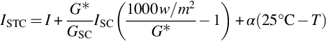
where ISTC is the current at STC, I the current as measured, T the temperature during the measurement, and α the absolute TC of short circuit current. G* is the (effective) irradiance at time of data acquisition of individual I–V data points, and GSC is the irradiance at the time of ISC measurement. This method is used to correct for unstable irradiance during the measurement. It is mandatory that the irradiance be measured point-by-point like current and voltage.
where VSTC is the voltage at STC, ISTC is the current at STC, V and I are the voltage and current as measured, RS is the series resistance, T is the temperature during the measurement, k is the curve correction factor, and β is the absolute TC of open circuit voltage.
The parameters k and RS are determined from measurements at different temperatures (like TCs) and different irradiances, respectively (for details see Ref. [15]). For very small corrections (few percentage points), they can be neglected. For larger corrections, it is possible to work with generic module type or technology specific values [17]. The values strongly differ between thin-film and crystalline silicon PV modules, and the suitability of generic values for thin-film PV module types must always be evaluated carefully.
2.2.7 Module stability
The considerations made so far assumed PV modules are stable with regard to their electrical parameters. A PV module can be considered as stable ‘if its electrical characteristics neither depend on its history of exposure to irradiance and temperature, nor on previous electrical bias or operating conditions, nor on combinations of these’ [18]. Strictly speaking, this is never really the case for PV modules, especially not for most thin-film PV modules. Depending on the state of the module, the determined STC parameters may be different after a certain amount of dark storage or exposure to light. This can imply either power increase or decrease. For significant interpretation of measured parameters, it is necessary to characterize the stability of a module (or module type) in terms of time scale, magnitude and external causes (irradiance, temperature and electrical operation). It is useful to differentiate between irreversible and reversible (metastable) changes of the module I–V curve.
Known (meta)stability effects depend on module technology, and were summarized, for example, in Refs. [18,19]. It must be noted that the most relevant stability or metastability effects depend on the PV technology group. A-Si is affected by the Staebler–Wronski effect which causes, on the one hand, severe light-induced degradation (LID) in the first (hundreds) of kilowatt hours of exposure but, on the other hand, allows for annealing of defects at higher temperatures. This is visible as seasonal annealing in the performance of PV systems. Chalogenide technologies (mainly CdTe and chalcopyrite technologies (CI(G)S)) are affected by dark storage. The power change induced by dark storage can be recovered by exposure to light. Table 2.2 summarizes the most important effects per technology (table reprinted from [18]).
Table 2.2
Reported impact of (meta)stability effects on module STC power
| c-Si | Amorphous silicon (a-Si, a-Si/a-Si, a-Si/μ-Si, triple junction) | CdTe | CI(G)S | |
| Initial light-induced degradation | Around 1% [20], up to 4% [19] | Often around 15–20% [21], but up to 35% [22]; takes 100 or more kWh to stabilize [23], stabilized power is dependent on exposure conditions [24,25] | 4–7%, but also power increase observed [26,27], superposition of recovery from dark storage and LID is possible | Both decrease and increase in the range of 1% to more than 10% observed [23,27], superposition of recovery from dark storage and LID is possible |
| Seasonal annealing | Not relevant | Amplitude of 3–6%, dependent on location and operating temperature [28–31], tends to be in the lower range for a-Si/μ-Si modules [32] | Not observed in published literature | Not observed in published literature |
| Sensitivity to unbiased dark storage (reversible by preconditioning) | Not relevant if module is stabilized | Not relevant if module is stabilized and kept in the dark at constant temperature | Several percent, up to 10% [23,27] | Several percent, up to 15% [23,27,33,34] |
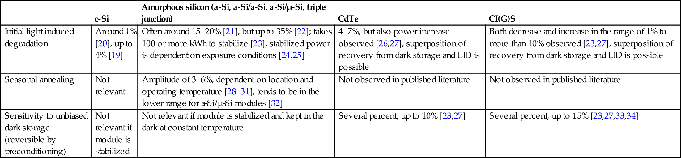
From D. Dirnberger, Uncertainty in PV module measurement—Part II: verification of rated power and stability problems, IEEE J. Photovolt. 4 (2014), 991–1007.
Summary of observed magnitude of stability problems in the mentioned literature, given by technology and group of effect. Note that all results are specific to material and processing of the modules, so that they can be transferred to behaviour of other module types of same technology only qualitatively and approximately.
There are several terms used to refer to stability effects or the methods to limit their impact. An overview on these terms according to [18] is given in the following:
• Preconditioning/pretreatment procedures: conducted in order to remove metastable effects. Such procedures involve exposure of the module to irradiance and/or temperature at electrical bias or in open circuit. Relevant especially for chalcogenide PV technologies (cadmium telluride, CI(G)S) that are sensitive to dark storage.
• Sensitivity to dark storage: modules change their STC power as a consequence of dark storage. Power loss is more common, but power gain has also been observed.
• Stabilization: Procedure conducted in order to permanently remove initial stability effects, such as LID. Modules are exposed to 1000 W/m2 in operation at MPP or open circuit until they are stable. The stability is determined either by subsequent I–V curve measurement in the laboratory (eg, every 43 kWh [35]) or by in situ I–V curve measurements.
• LID: Permanent degradation that occurs in the first tens or hundreds of kilowatt-hour exposure. Occurs for crystalline silicon (typically between 0% and 2%) and amorphous silicon (15–25% or more), and can occur for chalcogenide PV modules. For the latter, LID may be hard to determine because the power loss due to initial degradation could be masked by the power increase due to recovery from dark storage.
• Seasonal annealing: reversible change of module STC power in the field (increase in warmer months, decrease in colder months). Mainly observed for a-Si PV modules due to the Staebler–Wronski effect.
• Long-term degradation: power loss that occurs when modules are operated continuously, for example, as part of a PV system. See Ref. [36] for a summary of observed degradation rates.
One must be aware that the mentioned effects can influence the result of laboratory measurements, while the goal of measurements sometimes is to characterize these stability effects. Such measurements need to be planned properly, and it is important to consider the impact of stability effects depending on the timescale in which they occur (ie, cause the apparent PV parameters to change):
• ms: such very short timescale effects (eg, transient processes in the semiconductor structure) influence the I–V curve measurement itself, and, in extreme cases, may exclude the use of pulsed solar simulators. They increase measurement uncertainty and decrease reproducibility.
• Hours/days/weeks (eg, sensitivity to dark storage): the measurement result depends on the time that passed, for example, after dismounting the modules from an outdoor test set-up, or after a specific preconditioning procedure. Measurements must therefore be very well planned and documented, but are able to characterize the stability effects.
• Month/years: laboratory measurements can be used to characterize these changes without constraints, for example, long-term degradation of c-Si modules.
Solutions for stability problems are required for significant quality assurance. They depend on module technology and the purpose of the measurement. In Ref. [18], four different practical cases are explained:
• Verification of module power of new modules: The module power must be determined with initial effects removed, as the rated STC power must be representative of field operation. For crystalline silicon modules, this is typically tested by 20 kWh exposure (20 h, 1000 W/m2, operation in VOC; lower irradiance levels are allowed for outdoor exposure). For a-Si modules, the exposure time must be longer [35]. In situ I–V curve measurements during the stabilization period are recommended as this can considerably decrease measurement effort for determination of stability. Often, manufacturers of thin-film PV modules give indications of how the initial stabilization has to be conducted.
• Verification of power loss during accelerated ageing tests: The module power must be measured in the most reproducible way. Metastable effects can alter module power in between two measurements and must be dealt with under consideration of the specific characteristics of the module type under scrutiny.
• Verification of module power on field-exposed modules: Depending on the module technology and potential module-type-specific characteristics, sensitivity to dark storage (during transport) can affect the result.
• Calibration: above all, reference devices have to be stable. The short circuit current is often not or only little affected by (meta)stability issues, so that one solution can be to strictly use only the current for calibration. In cases where power is also used for calibration (eg, in some production lines), the module behaviour should be known very well.
As stability or metastability issues depend strongly on the detailed semiconductor composition and details in the production process, every module type must be looked at separately. For quality assurance purposes for large projects, it is reasonable to investigate the characteristics of one module type periodically. For the evaluation of the stability behaviour, comparison of indoor and outdoor measurements is essential. Fig. 2.6 shows an exemplary procedure of how a thorough investigation could be conducted [18].

2.2.8 Summary of influences on the I–V curve parameters ISC, VOC, PMPP, FF
For analysis of deviations between two measurement results for the same DUT, it is helpful to keep in mind which influences most affect which electrical parameters.
As the photocurrent generation depends on the incident irradiance, but not much on temperature, ISC depends on all mentioned aspects regarding measurement of irradiance. These are calibration, spectral mismatch and nonuniformity. Note that the calibration affects all measurements regardless of the characteristics of the DUT, while the other two also depend on module characteristics. ISC is a rather stable parameter, but can be affected by metastability issues for a-Si devices. VOC is affected mainly by temperature and, in the case of thin-film modules, by stability issues. When differences in FF are observed, this is typically related to contacting issues, capacitive effects and, in the case of thin-film modules, again stability issues. Differences in all mentioned parameters accumulate in differences of PMPP, as PMPP = ISC · VOC · FF. If a positive deviation in ISC is combined with a negative deviation in FF, this can lead to no deviation in PMPP. To judge on the overall quality of a comparison, it is therefore important to compare all parameters.
A summary of the most relevant influences per electrical parameter is given in Table 2.3. Note this represents the typical case, but can serve only as the starting point for a specific real case. The exact reason for deviations must be carefully analysed based on the exact measurement procedures that were applied by the involved parties. Examples for the interpretation of measurement results following this precept can be found in Ref. [37].

2.2.9 Measurement uncertainty for STC measurements
Measurement uncertainty, whether for I–V curve measurements or any other discipline, is information about the significance of the result of a measurement. The introduction to the Guide to the Expression of Uncertainty in Measurement (GUM) describes measurement uncertainty as an indication of ‘how well one believes one knows’ [38, p. 3] the true value of a quantity by the measurement result. The ‘true value’ is a theoretical concept and can never actually be known. Uncertainty in more detail is probabilistic information—the probability density function that is attributed to a measurement result shows the range of values around the measurement result which has a specific probability to contain the true value. To somewhat standardize the information included in the probability density function, the coverage probability7 is used. This is the probability that the true value lies within a specific interval, for example, the interval represented by the measurement result plus and minus the standard uncertainty associated with the measurement result. This interval is called coverage interval. Its magnitude depends on the selected coverage probability and the probability density function. Fig. 2.7 presents a simple example to demonstrate the introduced terms. It shows a measurement result, here the measured STC power of a PV module (250 W), and the attributed probability density function, here a Gaussian function. The standard deviation of the Gaussian function is equal to the determined standard uncertainty of, here, 0.8%. For a desired coverage probability of 95%, the Gaussian function requires the standard uncertainty to be multiplied with a coverage factor of approximately 2. The ‘expanded uncertainty’ is then 1.6%. The coverage factor depends on the probability density function and can often be determined only approximately.


It is important to understand the probabilistic character of measurement uncertainty in order to be able to correctly interpret measurement results under consideration of their uncertainty. Especially when evaluating differences between measurement results, or between measurements and data sheet specifications, one must be aware that a measurement result is not the absolute truth, but the best available estimate. Results that agree within the standard uncertainty can usually be looked at as essentially equal.
For the evaluation and quantification of measurement uncertainty, general rules are given by a framework of documents provided by the Bureau Internationale des Poids et Mesures (BIPM)8 [38–41]. These documents are available free of charge from the BIPM website9 and are also ISO standards [42–44]—except the International Vocabulary of Metrology (VIM) [41]. The process of measurement uncertainty evaluation is summarized in the GUM [39] in eight steps (see Section 8 of GUM; for a more basic and PV-related explanation see also [13], Section 2.4). These steps include identification, quantification, and combination of contributions to uncertainty. The key to sound uncertainty evaluation is that enough information about the measurand, the measurement procedure and equipment, and other influencing factors is gathered. In the context of PV module calibration, this concerns all influences that were discussed in the previous sections.
The first step according to GUM is to formulate a measurement equation, which expresses the relation between measurand (eg, ISC, PMPP and VOC) and input quantities (everything that influences the measurand, eg, irradiance, reference cell, spectral mismatch, temperature, etc.). Ideally, this equation analytically represents the relation between measurand and all input quantities. In praxis, this is rarely possibly, so the GUM suggests the following simplification (paragraphs 5.1.4 and 5.1.5 in Ref. [39]):
where Y is the measurand, ![]() and X1,0, X2,0, …, XN,0 nominal values, Xi the input quantities, N the number of input quantities,
and X1,0, X2,0, …, XN,0 nominal values, Xi the input quantities, N the number of input quantities, ![]() transformations (eg, changes compared to the nominal values) of the input quantities, and ci the sensitivity coefficients.
transformations (eg, changes compared to the nominal values) of the input quantities, and ci the sensitivity coefficients.
This equation expresses empirically how a specific change δi in an input quantity Xi propagates to the measurand. For example, the calibration value of the reference device is an important input quantity. According to Eqs (2.9), (2.12), it propagates directly to the STC short circuit current, that is, c = 1. Thus, δ of 1% in the reference device calibration would cause an error of 1% in the ISC. For the temperature influence, c is equal to the TC: the temperature difference ΔT from 25°C during measurement will cause (if no correction to STC is performed) a change in the measurand with a magnitude of ΔT times the TC.
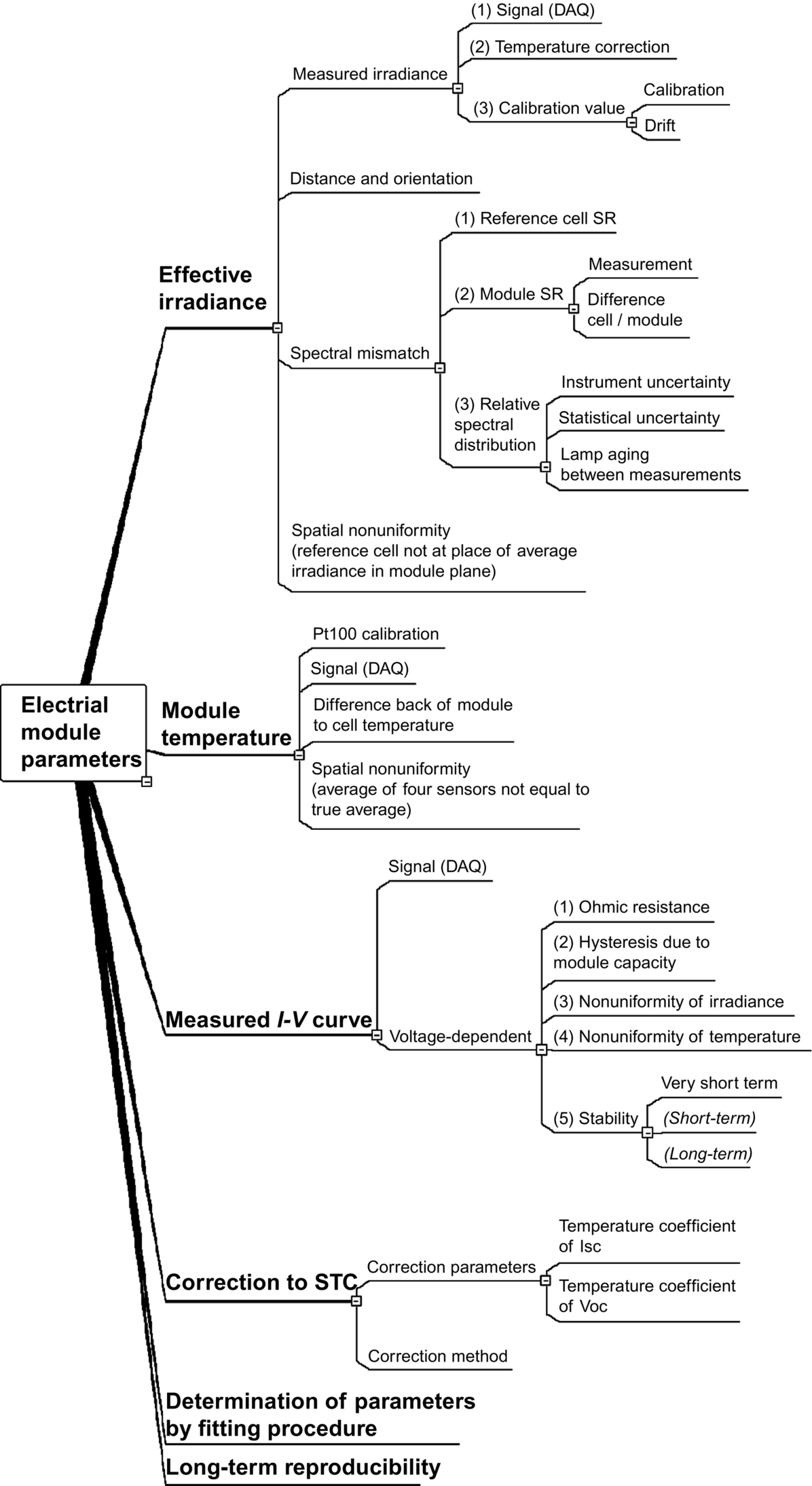
After having formulated the measurement equation, the estimated values of the input quantities must be determined (step 2). These are both quantities that result from the measurement under consideration (I–V curve, irradiance and temperature) as well as quantities that must be obtained from other sources (calibration value of reference cell, ambient conditions, spectrum of simulator, etc.). To visualize all input quantities, herringbone diagrams are helpful. As an example, Fig. 2.8 shows the most important input quantities as considered in the uncertainty evaluation by Fraunhofer ISE's module calibration laboratory CalLab PV Modules [8].
Then, the standard uncertainties of the input quantities must be determined (step 3). This is often an estimation based on calibration reports or characterizations of measurement equipment (eg, to determine that variability of the solar simulator spectrum) and the DUT (eg, the SR). Furthermore, possible correlations between the input quantities must be determined (step 4). A typical example for a correlation is the following: for determination of FF, both ISC and IMPP are required. These quantities both depend on irradiance and are thus correlated, which must be considered in the uncertainty calculation.
The result of the measurement is calculated using the formulated measurement equation (step 5). When the previous simplification (Eq. 2.14) is used, this step may be obsolete. If Y0 is already the corrected measurement result and other corrections are not made, the only purpose of Eq. (2.14) is to formally derive Eq. (2.15) for calculation of the combined standard uncertainty. It is important to keep in mind that, even if the changes δi are assumed to be zero, this does not mean that δi is without uncertainty. The combined standard uncertainty is determined using the following equation (step 6), assuming no correlations between the input quantities:
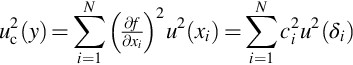
where ![]() are the partial derivatives evaluated at the expected values of Xi (sensitivity coefficients); uc is the combined standard uncertainty; and u(xi) are the standard uncertainties of the input quantities Xi (Eq. 10 in the GUM; here: xi = δi).
are the partial derivatives evaluated at the expected values of Xi (sensitivity coefficients); uc is the combined standard uncertainty; and u(xi) are the standard uncertainties of the input quantities Xi (Eq. 10 in the GUM; here: xi = δi).
If input quantities are correlated, an appropriate equation must be used (see GUM), or other, simplified methods to deal with the correlation must be applied. In the case of FF, for example, it is possible to determine the uncertainty for the quotients IMPP/ISC and VMPP/VOC instead of the uncertainty for the individual values, which implicitly considers correlations.
Uncertainty evaluation can consist of several subsequent steps of combining different contributions to combined uncertainties. For example, Fig. 2.8 shows that the combined uncertainty for the effective irradiance depends on contributions from the spectral MM, spatial nonuniformity and the reference cell calibration. The final combined uncertainty of the I–V curve parameters depends on the uncertainty of effective irradiance, module temperature, measured I–V curve, etc.
After having determined the combined standard uncertainty, the expanded uncertainty of the measurement result is calculated by multiplying the standard uncertainty with an appropriate coverage factor k (step 7). The coverage factor depends on the exact probability density function. This function is often not known, and is then assumed to be sufficiently well represented by a Gaussian probability density function. The coverage factor that is accordingly assumed is approximately 2, and the coverage probability approximately 95%. Finally, the measurement result is presented along with combined standard or expanded uncertainty (step 8). It should be kept in mind that an uncertainty evaluation is only valid when conditions during the measurement and characteristics of the DUT conform with the assumptions made during the uncertainty evaluation—for example, the spectral mismatch uncertainty depends on the SR of the DUT, and the nonuniformity influence is different for smaller and larger modules. Therefore, depending on the measurement equipment in use, it may be necessary to estimate some contributions to uncertainty specific to the DUT [8,37,45].
Detailed examples for measurement uncertainty budgets for PV module calibration which also include quantitative indications can be found in Refs. [8,46,47]. The lowest achieved measurement uncertainty for PV module calibration is 1.6% [8], with the largest contributions to uncertainty arising from reference cell calibration, spectral mismatch and spatial nonuniformity.
2.2.10 Importance of calibration and traceability
The role of the reference device calibration value in PV module measurement was explained previously (Eq. 2.9). It is easy to see that a change in the calibration value can shift the result of a PV module measurement to higher or lower current and thus power. For a consistent evaluation of the power of PV modules, it is thus important that the primary calibration procedures applied throughout the world achieve comparable results.
In general, national metrology institutes transfer the definition of SI and other units to accredited laboratories and to the market. In the case of PV, this is done by providing primary-calibrated reference cells. ‘Primary calibration’ (or, according to the VIM [41], ‘primary reference measurement procedure’) denotes a measurement procedure that produces a result with a specific unit without using a reference device with a calibration value with the same unit. Primary calibration procedures for PV devices transfer the measured radiated energy (in units of watts) to current generated by the PV device (in units of amperes). With a calibration value resulting from a primary calibration, the device becomes a ‘primary standard’. The calibration is transferred from PV cell to PV module by I–V curve measurement as described in the previous sections (using a primary standard as reference cell). PV modules (or cells) with calibration values from such measurements (‘secondary calibration’) are ‘secondary standards’. The calibration level is then further transferred by the creation of reference standards and working standards. For such measurements, a secondary standard is used to measure the irradiance instead of a primary standard. The pyramid in Fig. 2.9 depicts the multiplication of the calibration level from primary standards to working standards. While the definition of primary and secondary standards is strict, the use of the terms reference standard and working (reference) standard can sometimes differ. Manufacturers frequently also use the terms golden or mother module for the standards they use for creation of further working standards. The established calibration and recalibration regime is specific to the manufacturer or laboratory. It is important that every standard device used be somehow traceable back to a primary standard, as each additional transfer of calibration adds uncertainty, and the mere fact that a traceable standard is used as a reference device does not guarantee low uncertainty.
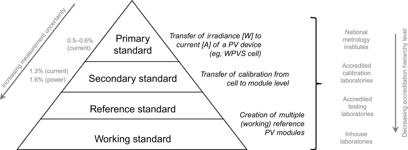
At the time of writing, primary calibration of PV cells is carried out by a small number of laboratories and national metrology institutes all around the world. The most important ones are the PTB (Physikalisch-Technische Bundesanstalt, Germany's national metrology institute), NREL (National Renewable Energy Laboratories, Golden, Colorado, USA), ESTI (European Solar Test Installation, part of the European Commission's Joint Research Center in Ispra, Italy) and the AIST (National Institute of Advanced Industrial Science and Technology, part of the Research Center for Photovoltaic Technologies in Japan). These laboratories use different indoor or outdoor methods, for example, the Differential Spectral Responsivity Method at PTB [48–51], the Solar Simulator Method at AIST [52,53] and ESTI [54], the Direct Normal Sunlight Method [55,56] at NREL and ESTI [57], and the Global Sunlight Method [58] at ESTI. A comparison of several primary calibration methods is included in Ref. [54]. The procedures are traceable to SI units (PTB) or to the World Radiometric Reference [59]. The currently lowest measurement uncertainty is provided by PTB (0.5–0.6%, k = 2 [48]). The international comparability of these procedures is traced by intercomparisons such as the WPVS [12,60,61].
Secondary calibration of PV modules is carried out by several laboratories all around the world. These are reference laboratories both for manufacturers and other service laboratories. Intercomparisons such as presented in Ref. [37] check on the comparability of secondary calibrations on module level.
While traceability is certainly most important for the reference device calibration, all measurement equipment used should be calibrated and traceable back to primary standards.
In parallel to the hierarchy in the traceability chain, the accreditation level of a laboratory is important (see Fig. 2.9). The accreditation represents the degree of third-party verification of the measurement equipment, procedures, and uncertainty estimation. The exact requirements to obtain accreditation as a calibration laboratory or testing laboratory may differ slightly from country to country, as each country has its own accreditation body (eg, DAkkS in Germany, UKAS in Great Britain, or ANSI in the United States). The national metrology institutes are usually part of the accreditation process, as they are the state organization responsible for measurement. In general, the accreditation level does not give information about whether a laboratory produces primary, secondary or working standards.
2.3 PV module characterization
2.3.1 Introduction of yield-relevant module characteristics
As mentioned previously, STC power is by far not the only important characteristic to assess PV module performance. The operating conditions span over a wide range of temperatures, irradiance levels, angles of incidence of the sunlight, and spectral distributions. The influence of these conditions on the energy produced depends on the corresponding module characteristics, which are:
• Irradiance dependency (or low light behaviour)
• Spectral response
• Angular response
• Thermal behaviour
In the following sections, state-of-the-art measurement methods for determination of these characteristics will be introduced. Furthermore, long-term stability of STC power and the mentioned characteristics is important. While long-term stability of STC power has been in the focus of many investigations [36], information about the long-term stability of the other characteristics is rare.
2.3.2 Measurement of temperature dependency: methods and challenges
The temperature dependency is determined by I–V curve measurements at a constant irradiance, typically 1000 W/m2, and different temperature levels. Therefore, temperature dependency measurements require the same set-up as for STC measurements and in addition the possibility to heat up and cool down the DUT. Typically, temperature chambers are used. The offered temperature range is at least 25–65°C; modern temperature chambers even offer ranges from 15°C to 75°C. Data obtained in the range of 25–65°C is, however, sufficient for most practical applications.
Compared to STC measurements, the measurement of the temperature of the DUT is even more important. Using a sufficient number of temperature sensors is mandatory in order to monitor and control the temperature nonuniformity over the module during all measurements. Normative guidance for TC measurement is included in the standards IEC 60891 Ed. 2 [15] and IEC 61853-1 [62] (measurements at different temperature levels).
Using a temperature chamber, there are, in principle, two ways for performing the measurement: either the module is heated up first and I–V curves are measured during cooling in specific temperature increments (eg, 1 K), or the module is heated up to selected temperature levels and kept there for each I–V curve measurement. In both cases, keeping nonuniformity within set limits is essential. A reasonable limit when using four temperature sensors is a difference of 2 K between minimum and maximum temperature.
The first method allows for taking more data points in reasonable time, but the accuracy is limited when the pulse duration is too short for the capacity of the DUT (compare Section 2.2.3). As the cooling process goes on continuously, each I–V curve must be finished within one pulse as otherwise the temperature will change too much (note that most simulators require at least 10–30 s between two pulses). Customized methods for temperature correction of each I–V curve point might solve this issue. The second method allows keeping the module at the selected temperature level for a longer time and thus conducting multiflash or section measurements. However, the number of points is limited for time reasons—it takes a while until the temperature has stabilized. Thus, an individual data point and its statistical measurement uncertainties can influence the overall measurement result relatively strongly.
The typical results of a temperature dependency measurement are TCs for the electrical parameters ISC, VOC, PMPP and FF. For each measured I–V curve, the parameters ISC, VOC, PMPP and FF are determined and plotted versus temperature in order to calculate the respective TC (Fig. 2.10). The TC can be reported either as absolute (ie, mV/K, mA/K, mW/K, etc.) or relative value. Relative values are calculated by dividing the absolute TC by the corresponding STC value:
where TC and XSTC are the TC and the STC value of the parameter under consideration, respectively.

The uncertainty of the absolute TC of an individual module is smaller than that of the relative TC, as the STC uncertainty does not contribute. Thus, important influences like calibration of the reference cell do not influence the uncertainty. However, the absolute TC varies depending on the module-specific voltage or power. Relative TCs eliminate this influence and can thus be used as generic values, for example, for different power classes of one module type on the datasheet or even for different module types of the same module technology (eg, standard c-Si). In the case of metastable modules (Section 2.2.7), the TC can be influenced by temperature-induced metastable changes of the module state. For example, annealing that takes place while the module is heated up to different temperature levels for subsequent I–V curve measurements can reduce the apparent TC: STC power increase due to annealing partly makes up for the power decrease due to rising temperature. The exact influence depends on the measurement method and the module behaviour and can thus not be quantified on a general basis.
Some module types exhibit nonlinearities, which typically show only in measurements over a larger temperature range (eg, 15–75°C; compare Fig. 2.13). Typically, these are quite small and can be neglected—especially considering that simulations are usually performed under the assumption of a linear temperature change, that is, TC is constant over temperature. If larger nonlinearities occur, it may be necessary to use different TCs depending on the temperature range under consideration. In the case of metastable PV modules, nonlinearities can appear as a consequence of the metastability.
Uncertainty of relative (linear) TCs is currently estimated to be around 25% for ISC (the influence is very small and thus difficult to measure) and around 5–10% for VOC and PMPP, although commonly agreed-on methods for determination of this uncertainty still have to be developed. The fact that TC is a value derived from a set of other values limits application of the GUM [39] and requires approaches such as Monte Carlo methods [40]. Prerequisites for accurate and precise results are sufficient temperature uniformity, accurate temperature measurements and high reproducibility of measurements.
2.3.3 Measurement of irradiance dependency: methods and challenges
The irradiance dependency of a PV module is often referred to as ‘low light behaviour’. It is usually measured at 25°C in a range of 100–1000 W/m2 in 100 W/m2 increments. Some simulators allow for irradiance levels of up to 1300 W/m2. The measurement result consists of a set of measured I–V curves. The ‘low light behaviour’ is typically reported as ‘relative efficiency’, which is the measured efficiency normalized to the efficiency at 1000 W/m2. Like the relative TC, this allows for easy comparison between module types or modules with different STC power (Fig. 2.11).


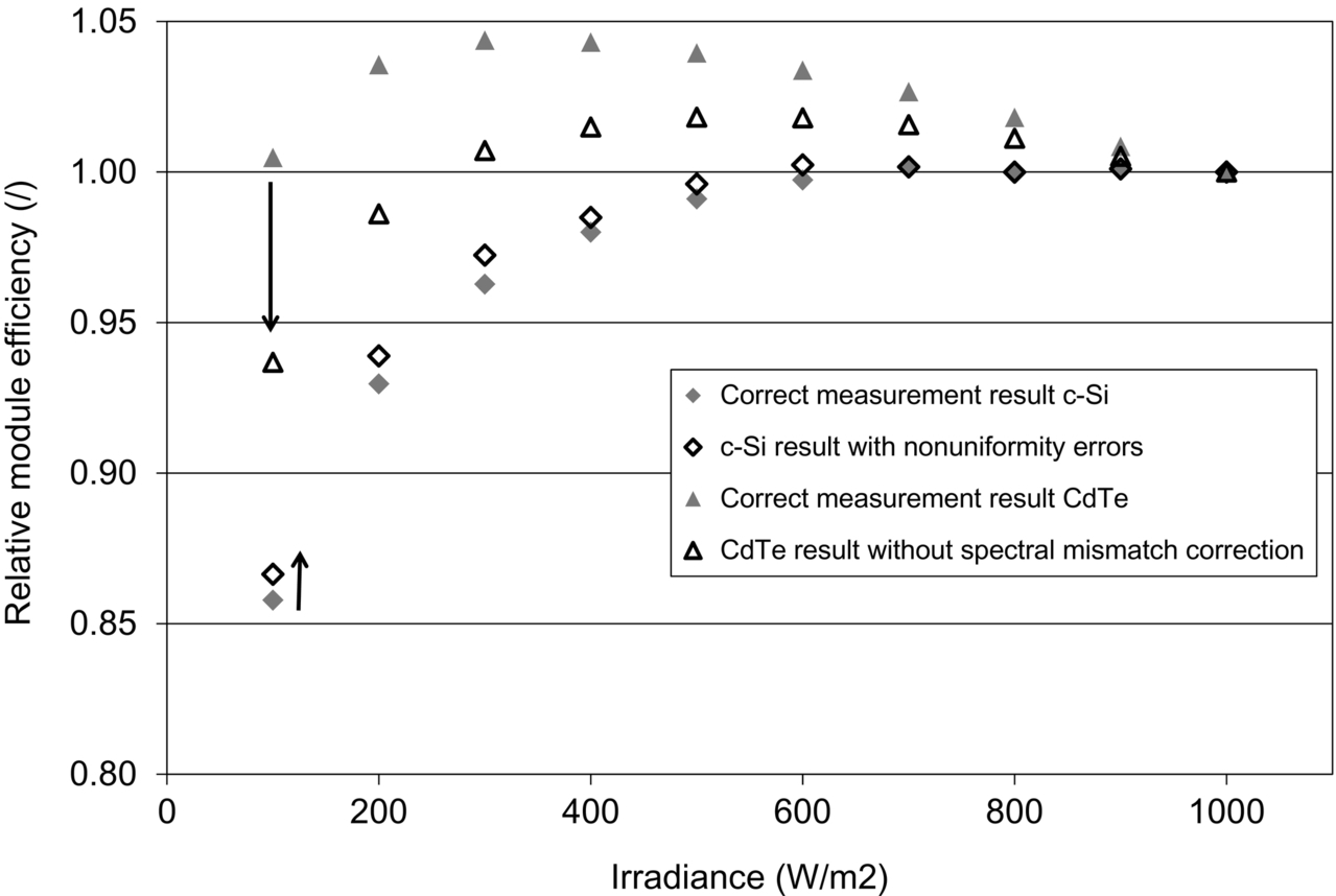
In addition to the STC measurement equipment, the possibility of changing the irradiance level is required. Normative guidance can again be found in the standards IEC 60891 Ed. 2 [15] and IEC 61853-1 [62]. The technical challenge of irradiance dependency measurement is to reduce the simulator irradiance without changing other light characteristics such as nonuniformity or spectral irradiance. Otherwise, the apparent irradiance dependency is a combined effect of the actual irradiance dependency and alterations induced by the dependence on spectral irradiance or nonuniformity. State-of-the-art solar simulators are optimized for measurements at STC, so that, typically, at least one light characteristic does change. This increases measurement uncertainty. If such influences are not recognized and corrected, this has consequences for the quality of the measurement result: the relative efficiency can systematically appear better or worse (Fig. 2.12, [63]).
There are mainly two established concepts for reducing irradiance: either the power for operating the simulator lamps is reduced or the produced light is reduced by means of filters. Reducing lamp power increases the share of higher wavelength in the light, so that the spectrum changes with irradiance. Especially for large differences of SR of reference device and DUT, this can lead to large systematic errors. Spectral mismatch corrections specific to each irradiance level can solve this issue. Using grey filters usually affects nonuniformity, while keeping the spectral distribution constant on the whole (note that often a combination of grey filters with slight changes in lamp power is necessary to perform measurements in 100 W/m2 increments). The effect on nonuniformity strongly depends on the quality of the grey filters, so that it is mandatory to measure the nonuniformity with each filter set in use (Section 2.2.2). With high-quality filters, the nonuniformity can usually be kept below or around 2% for typical module areas of around 2 m × 1.1 m.
Uncertainties for ‘low light efficiency’ are to date reported mainly for the 200 W/m2 efficiency (the absolute value), and are in a range of 3.5–5% depending on the laboratory. For the relative efficiency, which is used for simulations, uncertainties are smaller because systematic influences like reference cell calibration are removed due to the normalization. The uncertainty is dominated by effects that influence measurements at different irradiance levels in a different way, such as shown in Fig. 2.12. It must be kept in mind that this influence is again specific to characteristics of the DUT. Furthermore, the apparent irradiance dependency may be influenced by module metastability, so that it is recommended to perform measurements after preconditioning/stabilization procedures whenever in doubt.
2.3.4 Power rating measurements according to IEC 61853-1
Temperature and irradiance dependency are typically measured at 1000 W/m2 and 25°C, respectively. For yield predictions and module simulations (Chapter 4), the data are also used to describe module behaviour at different combinations of irradiance and temperature levels, that is, the influences are assumed independent. In order to be able to verify this assumption, the power rating matrix suggested in IEC 61853-1 [62] foresees measuring I–V curves at different combinations of irradiance and temperature, so that, for example, the low light behaviour is available at several temperatures (Fig. 2.13).


The measurements are carried out with a simulator that is capable of reaching the required irradiance levels and has a temperature chamber. Some simulator manufacturers offer comprehensive software solutions to carry out these measurements automatically.
2.3.5 Measurement of SR: methods and challenges
The SR(λ) is the module characteristic that describes the dependence of photocurrent generation on the wavelength of the incident irradiance. It is related to the external quantum efficiency EQE(λ) as follows:
where h is the Planck constant, c is the speed of light and EQE(λ) is the wavelength-dependent EQE ([2], p. 12).
As was mentioned before, the SR of a module plays an important role in the achievable measurement uncertainty. As this data is required for spectral mismatch correction, the measurement is very often part of module calibrations.
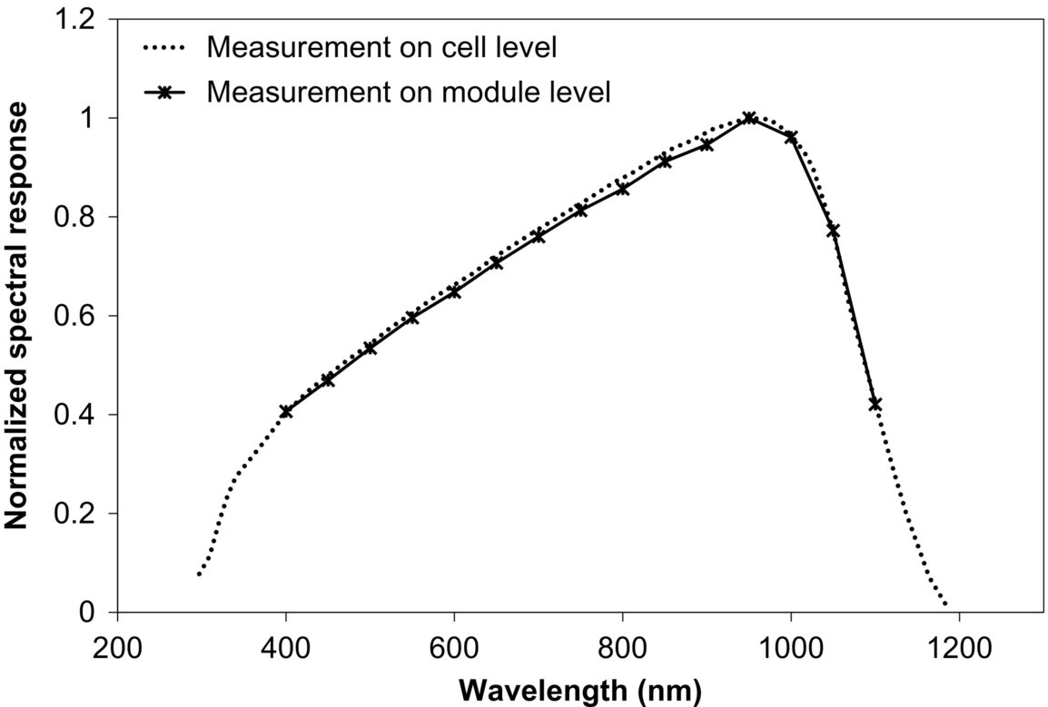
Measurements can be carried out on mini modules with the same cells, encapsulation, backsheet and glass as the full-size module under investigation. To exclude any effect from increased reflections, the mini module should consist of 3 × 3 cells with only the middle cell electrically connected. Alternatively, full-size modules can be opened up on the back side and one individual cell can be connected. SR measurements on cell level still have somewhat lower uncertainties than on module level (around 2–3% [64] compared to around 5% [65] in the range of approximately 400–1000 nm), but sufficient agreement is achieved in comparisons, as shown in Fig. 2.14.
For full-size modules, two different methods to measure the SR exist. The first one measures SR(λ) with the full module illuminated with quasi-monochromatic light (wavelength band with a width of around 50 nm or less), using a pulsed solar simulator with bandpass filters [66]. No bias light10 is applied, which limits the application of the method for nonlinear PV modules. The nonuniformity of the quasi-monochromatic light has an important influence on the measurement uncertainty. The nonuniformity can cause different cells to limit the measured current of the module. A measurement uncertainty analysis for this method was presented in Ref. [65].
The second method measures SR(λ) with only a small spot on the module illuminated with monochromatic light [67], and the other cells of the module flooded with bias light.
Recommendations for SR measurement on the module level are also included in the draft IEC 61853-2 [68] by reference to IEC 60904-8, Ed. 3.0 [69]. Guidance on measurement of multijunction modules can be found in Refs. [70,71].
2.3.6 Measurement of angular response: methods and challenges
The angular response of a PV module describes its relative reflection behaviour at nonperpendicular irradiance. One can speak of the ‘relative transmission’,11 which is measured via the short circuit current of the PV module (see also IEC 61853-2 [68]):

where τrel is the relative transmission and AOI the angle of incidence.
A set-up is required that allows for rotation of the DUT. As a consequence of the rotation, one part of the module will move closer to the light source than the other, and will thus receive more irradiance.12 For typical solar simulators, this increases the nonuniformity over the whole module to an unacceptably high level. Therefore, the measurements must be performed with respect to one single cell. The axis of rotation must be the middle axis of the cell, or the part thereof, that is measured.
Four methods exist for determination of the relative transmission according to Eq. (2.18) in the laboratory:
• Measurement of the short circuit current of a mini module (eg, nine cells) with only the middle cell electrically connected, with identical design compared to the full-size PV module under investigation (with regard to cell, encapsulation, and glass, etc.)
• Measurement of the short circuit current of a single cell of the module under investigation. The cell is contacted through the backsheet. The disadvantage of this method is that the module is damaged and not suitable for further use.
• Measurement of the short circuit current of the full-size module with one shaded cell [72]. Approximately half the cell is shaded, so that the current of this cell will limit the current of the module and thus the measured short circuit current at the module terminals is the current produced by the shaded cell. The bypass diodes of the modules have to be removed.
• Measurement of I–V curves of the full-size module with no shading and with one shaded cell. The current value used for determination of relative transmittance is the current where both I–V curves have their intersection. Details on the evaluation can be found in Ref. [73].
Furthermore, the IEC 61853-2 [68] also includes an outdoor procedure.
The main contributions to uncertainty are the determination of the AOI and the effect of both stray light and the directional distribution of the light. An error of 1 degree in the determination of AOI at a nominal angle of 60 degrees causes a difference of around 3% in the relative transmission. The effect from stray light or directional distribution depends very much on the solar simulator in use.
2.3.7 Thermal behaviour
An important factor for the performance of a PV module in reality is the operating temperature that sets at specific conditions. The operating temperature depends on the thermal equilibrium that attunes, that is, on the incident irradiance, the ambient temperature, the wind speed and direction, and also the efficiency13 and construction of the module. As it is difficult to analytically describe this dependence and to experimentally determine relevant factors, so far the ‘thermal behaviour’ of a module has been reported using the nominal operating cell temperature (NOCT) determined according to IEC 61215 [74].
The NOCT test is performed outdoors, the module being mounted in an open rack at a 45-degree tilt angle and operated in open circuit. Module temperature is monitored along with irradiance, ambient temperature and wind speed. NOCT is the temperature determined according to specific rules for reference conditions of 800 W/m2, 20°C ambient temperature and 1 m/s wind speed.
The results from this procedure were found to be location and test set-up dependent, so that the NOCT concept and the method are questioned among scientists [75–77]. For example, NOCT values indicated on the data sheet tend to differ strongly (up to 10 K) between different module types with same cell technology and similar construction, but scientific results presented in Ref. [75,76] suggest that the actual difference is negligible in such cases. Furthermore, PV modules have higher operating temperatures (several degrees) when operated in open circuit compared to MPP.
An alternative procedure to overcome these limitations is suggested by Koehl et al. [76]: a realistic module operating temperature (ROMT) shall be determined for straightforward comparison of module types, along with model parameters for description of the correlation between irradiance, ambient temperature, wind and the module operating temperature. The parameters could be used much better for simulation of module temperature under different conditions in PV performance predictions (Section 2.5), and would thus enable differentiating modules also considering their thermal behaviour in future.
While one could think of methods to determine NOCT or a comparable parameter in the laboratory, for example, using wind tunnels, controlled air temperature and suitable solar simulators, efforts to develop such methods are not known to the author at the time of writing.
2.3.8 Outlook on special requirements for outdoor calibration and characterization
In the previous sections, the calibration and characterization of PV modules was described with a focus on laboratory measurement methods. All the measurements can also be performed outdoors, and the applicable rules are the same. As outdoor measurements depend on the current weather conditions and the local climate, the specific challenges are a little bit different:
• I–V curve measurement: As the sunlight is constant light, there are no issues regarding sweep speed and capacity effects, as long as appropriate measurement equipment is used and as long as conditions are stable (eg, no moving clouds).
• Irradiance measurement: For outdoor measurements, pyranometers can be used as an alternative to reference cells; however, this increases uncertainties due to differences in spectral and angular response between reference device and DUT. Both for pyranometer and reference cell, care should be taken that the temperature has stabilized and that an appropriate signal temperature correction is applied. Nonuniformity of natural sunlight can be much better than in the laboratory, but this also depends on the exact location where the measurements are carried out (reflections from the surroundings can have a negative impact).
• Spectral distribution: Depending on location, time, weather and atmospheric conditions, there can be significant differences between the reference spectrum and the solar spectrum (see eg [78,79]). Therefore, the spectrum of the sun should be recorded and a spectral mismatch correction should be performed.
• Temperature: The determination of the correct module temperature is one of the largest challenges in outdoor measurement. As the irradiance will heat the DUT, the usual approach is to keep the DUT in an air-conditioned environment at a temperature somewhat below 25°C until directly before the measurement, and then make subsequent measurements during the heating up. To avoid making measurements while the temperature changes (transient processes negatively affect the temperature nonuniformity over the module and the difference between the temperature at the backside of the DUT and the actual cell temperature), one could also let the temperature stabilize and then perform corrections to STC (Section 2.2.6). In that case, uncertainties due to the correction, especially due to uncertainties in the TC, occur [17].
• Correction to STC: If conditions are stable and close to 1000 W/m2, the situation is very similar to laboratory measurements. If this is not the case, the correction and especially the determination of the relevant parameters play a much larger role [17].
The great advantage of laboratory measurements is that conditions can be controlled and are independent of the weather and climate, which allows for very high reproducibility of measurements. Nevertheless, outdoor measurements can be as accurate and precise as laboratory measurements, if performed with the right level of expertise and at appropriate conditions. In intercomparisons, very good agreement was achieved between laboratory and outdoor calibration [37]. For new PV technologies or technologies that are sensitive to specific characteristics of solar simulators (eg, multijunction modules to simulator spectrum), outdoor measurements can offer a possibility to verify laboratory measurements.
2.4 PV module characterization in praxis for the purpose of quality assurance
2.4.1 Variability of module characteristics between modules of the same type
While the preceding sections contained descriptions of measurements of one individual module, it is important to keep in mind that characteristics can vary between modules of the same type. Thus, measurements of one individual module provide insufficient information about the quality of a whole batch of modules. In the following, the relevance of variable module characteristics for quality assurance is discussed.
First of all, the STC power varies among modules of one type due to cell power and the module production process. Typically, modules are binned to power classes with a width of 5 W, for example, 250, 255 Wp, etc. They can be ‘plus-binned’, that is, class 250 Wp includes only modules with STC power > 250 Wp. Alternatively, symmetrical binning is common, that is, class 250 Wp contains modules with STC power of 250 ± 2.5 Wp. The STC power here is the power measured at the end of the production line, with production line solar simulators. These measurements are typically less accurate than measurements in a laboratory and are especially affected more strongly by statistical influences. The STC power of a whole batch of modules is best determined by using proper sampling procedures, which is described in Section 2.4.2.
Module characteristics that are mainly determined by physical properties of the semiconductor, like SR and TC, typically do not vary strongly within one module type, and not even within one type of semiconductor. The low light behaviour additionally depends on module production-related influences, such as series resistance, so that larger variations can occur. For a high-quality module type this is, however, not expected. Typically, the variation is not larger than measurement uncertainty limits, meaning it is unclear whether variations are actual module-related differences or measurement artefacts. Fig. 2.15 shows the typical range for low light behaviour and TCs of standard c-Si PV modules according to measurements by Fraunhofer ISE. For thin-film modules, one must consider that module characteristics can vary quite a lot within the same technology group (eg, CI(G)S) [13].

The reflection behaviour is dominated by the air-glass interface and should thus not vary between modules of one type. However, extensive data to verify this do not yet exist.
Reasonable sample sizes for module characteristics are around 10–25 modules for STC measurements, 5–10 for low light behaviour and 1–3 for TC, spectral and angular response measurement. Regarding sample size, there is always a trade-off between significance of the result and costs for the measurements. The optimum depends on the specific situation. For quality assurance for thin-film modules or new PV technologies, rather higher sampling sizes are recommended.
2.4.2 Sampling schemes for STC power verification
Verification of STC power presents one of the most important steps of quality assurance when purchasing larger amounts of PV modules [80,81]. As not all modules can be measured by independent laboratories for time and cost reasons, a sample for the STC power verification must be selected.
In order to understand the underlying challenges, the following terms must be clarified:
• Flashlist: the list of STC power as determined by the module manufacturer in the production line (this measurement is the basis for binning modules to power classes). The flashlist values may include any manual offsets the manufacturer might have added, for example, a security margin in order not to overrate modules.
• Selected sample: the modules that were selected randomly or systematically for measurement in an independent laboratory. Only for this sample, measurements of STC power both by the manufacturer and the independent laboratory are available.
• Rated power: The power bin the modules were assigned. This value is constant for all modules of one type and power class, while the flashlist power is not.
The standard approach is to select a sample randomly, and to compare the STC power determined by an independent laboratory with rated power. When the average STC power of the sample is above or around rated power, the whole batch of modules is assumed to comply with the STC power rating by the manufacturer. Fig. 2.16 demonstrates why this can be misleading: The STC power according to the flashlist varies over the whole batch within the borders of the power bin width. If the sample is selected randomly, the modules might by chance all be picked from the range of higher power values, instead of, as shown in the figure, equally distributed over the whole range of power values. When the measurement performed for verification in an independent laboratory reveals that the correct power is approximately equal to the rated power, the situation seems ok. What is not considered by this analysis is the difference between the actual STC power and the flashlist power, which can be several percent: while modules with rather higher power still meet the rated power, this is not the case for modules with lower power. As a consequence, the conclusion regarding whether or not a batch of modules is accepted depends also on which modules were selected.
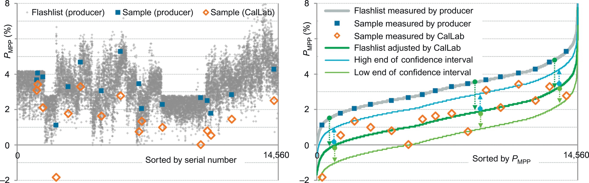
To prevent such kind of misinterpretations, the sample is best selected systematically [82], especially if large batches of modules are purchased. The procedure presented in Ref. [82] consists of the following steps and is shown in Fig. 2.16:
• Obtain flashlist of the batch of modules
• Determine average module power according to flashlist
• Select a number of modules (at least 10) out of the flashlist that are spread over the whole power and serial number range, and whose average power is equal to the average power of the flashlist (this is done using an algorithm)
• Measure the selected modules
• Determine the difference between the average measured power and the average flashlist power of the sample
• Adjust the flashlist by the difference and compare the adjusted flashlist average with rated power
For the example shown in Fig. 2.16, the rated power (0%, power is shown as deviation from rated power) is met by most of the modules and the batch can be accepted. The statistical spread in the difference between laboratory and flashlist value demonstrates that the sample cannot be arbitrarily small.
Alternatively, statistical evaluation procedures for module selection can be applied [83]. Here, the sample size is selected with the aim to achieve a specific probability for rejecting the batch while it is ok, or accepting the batch while it is not ok. Depending on the shape of the distribution of the STC power values in the flashlist, the necessary sample size can still become quite high.
2.5 Future trends and perspectives
In the future, PV module characterization may see twofold developments.
First, measurement uncertainties will decrease. Measurement uncertainty for STC measurements can decrease to values as low as 1.2%, assuming a reduction of uncertainties in primary calibration and SR measurements [8]. Improvement regarding uncertainties of characterization measurements will be driven by more detailed analyses and subsequent optimization of measurement equipment and more sophisticated methods to evaluate measurement uncertainties.
Second, measurement equipment for module characterizations such as spectral and angular response will become more available and/or easier to use. As a consequence, more information about module characteristics apart from low light behaviour and TCs will become available, which offers new ways for energetic module optimization and for decreasing uncertainties also in simulation. Furthermore, measurement equipment will be developed for characterization of emerging PV technologies, such as bifacial PV modules.