Concentrating photovoltaic systems
M. Steiner*; T. Gerstmaier†,a; A.W. Bett* * Fraunhofer Institute for Solar Energy Systems ISE, Freiburg, Germany
† Soitec Solar GmbH, Freiburg, Germany
a Formerly Soitec Solar GmbH
Abstract
The first section of this chapter introduces the principles of concentrating photovoltaic (CPV) technology. Since there is a huge diversity in system designs, the most common principles are outlined and examples for CPV systems are presented. The second section discusses the most important impacts on the performance of CPV systems. In contrast to standard photovoltaic (PV), the influence of the cell temperature on the output power is much less important. On the other hand, multijunction solar cells are used in high-concentration systems and therefore daily and seasonal changes in the spectrum have a stronger impact on the energy output compared to flat-plate PV. However, it is discussed that these effects must be seriously considered for the instantaneous power output but over a full year of energy production there is an averaging effect and the most dominant influence remains the irradiance. Sections 10.3 and 10.4 deal with the evaluation of CPV technology. Here, standards are an essential prerequisite. International Electrotechnical Commission standards for CPV technology are currently under development and drafts are already published. The sections give insight into the standards and detailed information about the benefits of these standards and provide examples of how to use them. Further, recent results of module, system and power station evaluation, applying these standards for the first time, are presented.
Keywords
Concentrator photovoltaics (CPV); Performance; Impact factors; Energy yield; Standardization; Prediction
10.1 General overview and description of CPV systems and technologies
Concentrating photovoltaic (CPV) technology is a recognized path to lower the cost of solar-generated electricity. The basic idea behind this technology has been pursued for many years, ie, reduce the comparatively expensive semiconductor material in a module. While in a standard flat-plate photovoltaic (PV) panel, the area of the solar cell collects and converts the sunlight in one unit, in CPV these two functions are separated into two units. The sunlight is first collected on an area which is an optical element. This optical element guides and therefore focuses the sunlight onto a smaller area, which is a tiny solar cell acting as a conversion unit. In this way, and as shown in Fig. 10.1, the light is concentrated and thus the intensity of the sunlight on the solar cell increases. In CPV the concentration factor is of importance. It indicates roughly how much semiconductor area is substituted for by an optical element. Two definitions are used for the concentration factor. One is based on the geometrical concentration (see Eq. 10.1) the other on the power concentration (see Eq. 10.2). Both are connected by the optical efficiency.


The optical efficiency accounts for losses in the optical element. These losses could be due to reflection, but also due to refraction, chromatic aberration or other optical losses. Typical practical optical efficiencies are in the range from 78% to 90%. It must be noted that the optical efficiency depends also on the concentration level. Higher concentration factors reduce the optical efficiency for a given optical element. However, there is a wide variety of different optical elements. In commercially available CPV systems today, the preferred primary optical elements are Fresnel lenses or mirrors. Frequently, a secondary optical element is implemented and this is typically mounted directly on the PV receiver area; see Fig. 10.2.

This secondary element helps to either increase the concentration factor further or to increase the acceptance angle of the CPV system. The acceptance angle of a CPV system defines the sector of the sky from which the sun's rays are collected and converted into electricity. For low concentration factors < 30 × it is up to 5 degrees, whereas for high-concentration ratios > 500 × it is in the range of 0.3–1.0 degrees. Thus, CPV uses preferably the light coming out of the direct solar disc, ie, the direct sunlight. Therefore, for rating CPV cells, modules and systems the AM1.5d(irect) reference spectrum, as defined in International Electrotechnical Commission (IEC) 60904-3, is used. Since the module can only use direct sunlight, the module area must be always vertically aligned to the sun's disc. Therefore, the CPV technology needs a tracking system to follow the sun precisely; see also Figs 10.4 and 10.5. The need for tracking increases the system complexity but results also in the benefit of a favourable, more rectangular daily energy production profile, which is visualized in Fig. 10.3.

The high variability in the choice of optical elements, tracking strategies and solar cells leads to a wide diversity in proprietary system designs. At any rate, the concentration factor is a possibility for categorizing the CPV systems adequately. Currently, two categories must be mentioned:
1. Low concentration system with concentration factor above 1 up to 30 × (LCPV).
2. High-concentration systems with concentration factors > 300 × (HCPV).
It might be surprising that no systems with concentration factors between 30 × and 300 × are on the market, but as it turns out, these systems are not yet cost-competitive.
The LCPV systems typically use modified Si solar cells, one-axis tracking and often a parabolic trough mirror. However, copper indium gallium selenide solar cell-based cells and linear Frensel lens collectors are also used. A typical LCPV system developed by the company Sunpower is shown in Fig. 10.4. For HCPV, two-axis tracking is mandatory. High-efficiency multijunction solar cells are used in these systems. The vast majority of the HCPV systems use Fresnel lenses as primary optics. This leads to the so-called point-focus design, ie, each Fresnel lens is placed directly over a small solar cell. The small solar cell is mounted on a heat spreader which distributes the heat very effectively. This cooling technique is called passive cooling. Fig. 10.5 shows a photo of a Fresnel lens type point-focus system and the schematics of the working principles.


Another approach for HCPV systems relies on active cooling. Active cooling increases the system complexity but a good benefit results from using the excess heat. So-called HCPVT (T means thermal) systems cogenerate heat and electricity. In this manner, sunlight conversion efficiencies beyond 70% are achieved [1]. Such systems use several tenths of a square-metre sized parabolic-shaped mirror to concentrate the sunlight onto PV receiver areas of several tenths of a centimetre squared. As receivers are commonly water cooled, densely packed PV arrays are used. A photo of such a system is shown in Fig. 10.6. Even larger PV receivers are used in solar towers, where many mirrors focus the light on a tower. The first solar tower demonstration systems have been set up [2] and prove the principles of this technology.

Today, the CPV market is clearly dominated by HCPV technology. As reported [3], the total installed capacity of HCPV is 314 MW whereas the capacity of LCPV is 26 MW. Obviously, the total installations of CPV systems are three orders of magnitude below standard flat-plate PV technology. Thus, CPV technology is just starting to enter the market. A very essential milestone to support the market entrance was achieved when the first IEC standard 62108, Design Qualification, was published in 2007. Further IEC standards have been developed in Technical Committee 82, Working Group 7 (TC82, WG7) and are now introduced. Some very important standards are the definition of the standard testing conditions for CPV technology and the procedure for rating of the systems, ie, the IEC62670 series. The background for these standards is more thoroughly explained in the following sections.
One specific feature in the HCPV system is the use of multijunction solar cells, which provide the highest solar conversion efficiency. Solar cells with efficiency of 46% have been elaborated in the laboratory [4] and industrially fabricated solar cells with efficiencies beyond 40% are commercially available in large quantities [5]. The industrial standard cell is a triple-junction device based on the material composition of GaInP/GaInAs/Ge. The 46% record efficiency value was achieved with a four-junction cell based on GaInP/GaAs//GaInAsP/GaInAs using wafer bonding technology. There are many triple, quadruple, and up to sixtuple multijunction solar cell architectures under research applying a variety of different production technologies. An overview can be found in Ref. [6].
However, the internal series connection of these solar cells makes precise measurement and characterization more challenging and requires new sun simulators [7]. For application in concentrator modules, not only are the laboratory measured solar cell characteristics of importance, but also the optical transmission function of the concentrating optics must be respected. In total, it has been shown for CPV modules that the sensitivity for changes in the spectral distribution of the sunlight is increased compared to flat-plate standard PVs. But eventually the yearly energy production is the only real measure that counts. Extremes can be found, but due to many daily and seasonal changes of the sun spectrum, the statistics lead to a smoothing effect. Several studies have been conducted investigating the influence on system performance of different sun spectra associated with different sites and modified (ie, site optimized) cell architectures [8]. The maximum difference in the yearly energy yield was found to be 3%. Thus, site-specific adapted solar cell designs can lead to a small improvement. At any rate, the existing excellent performance prediction models consider the influence of the spectrum; see also Section 10.3.
Aside from many specific details, CPV cells, modules and systems achieve the highest power output per area. Assuming the same aperture area, HCPV technology produces nearly twice the power compared to flat-plate PV. This proves that CPV technology is a high-efficiency technology. Moreover, further progress and higher output power can be expected in the future; see Fig. 10.7.

10.2 Impact factors on CPV performance
In silicon flat-plate PV the two highest impact factors on module performance are irradiance and solar cell temperature. For CPV the irradiance is the highest impact factor as well. But the influence of the cell temperature on CPV module performance is much lower compared to silicon flat-plate PV [11]. The second highest impact factor in CPV is not the cell temperature; it is the spectral distribution of the irradiance. The impact of the spectral distribution on module performance results from the use of multijunction solar cells. Multijunction solar cells consist of several subcells with different bandgap energies which are internally series connected. Each subcell absorbs light in a different wavelength range. In this manner, the sunlight can be more effectively used, ie, the solar cell efficiency is drastically increased. However, a change in spectral distribution of the irradiance, which occurs during every day and across the year, immediately alters the current generation in the individual subcells. For instance, assume two spectral distributions A and B with the same integral value of irradiance. Under spectral distribution A, all subcells in the multijunction solar cell produce the same amount of current, whereas under spectral distribution B one subcell produces much less current while the others produce more. Since the subcells in the multijunction solar cells are connected in series, the short-circuit current of the multijunction solar cell is limited by the subcell with the minimum current generation. As a consequence, the current of a solar cell measured under spectral distribution A can have a much higher value than for the same solar cell measured under spectral distribution B, even though spectra A and B have the same irradiance value. This is the reason why in a CPV application the impact of the spectral irradiance distribution has to be considered.
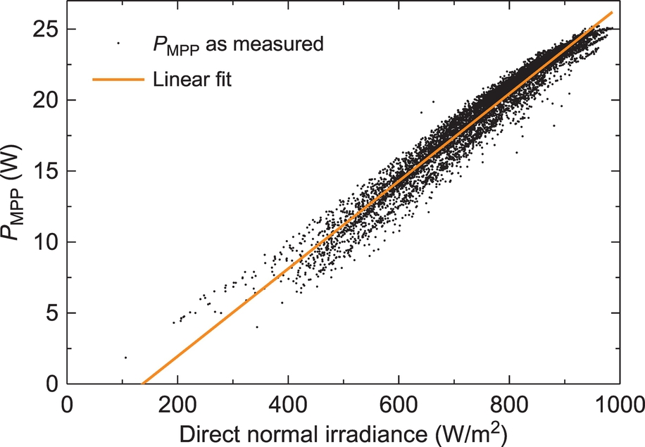
The integral value of the spectral irradiance distribution is measured in a similar manner as that for flat-plate PV by using a pyrheliometer. A pyrheliometer has the same operating principle as a pyranometer, but measures the irradiance only in an opening angle of ± 2.5 degrees. Thus, a pyrheliometer has to be mounted on a sun-tracking unit. The output of the pyrheliometer is called direct normal irradiance (DNI), which is the absolute integral value of the spectral irradiance distribution. Fig. 10.8 shows the dependence of module power output on DNI, using as an example a FLATCON-type CPV module [12] with lattice-matched triple-junction [5] and silicone-on-glass lenses [13]. The data were measured in one full year of operation at Fraunhofer ISE in Freiburg, Germany. Fig. 10.8 shows a linear fit to the data to underline the linear dependence of power output and DNI. The variation of the measured data points from the straight line of the linear fit is around ± 10%. This ± 10% variation is due to other impact factors such as the spectral irradiance distribution, temperature of cell and lens, module and tracker alignment.
The relative variations of the spectral irradiance distribution have to be measured with additional equipment as well as the pyrheliometer. The ideal method to measure this distribution would be to use a spectral radiometer with high resolution. The disadvantage of spectral radiometers is their high costs in combination with high measurement uncertainty when performing long-term measurements in a wide range of wavelengths. For CPV, typically the wavelength range of interest is between 250 and 1800 nm. Therefore, in CPV, component/isotype cell sensors [14–16] are used to quantify the impact of the spectral irradiance distribution on module performance.
The component sensor consists of multijunction subcells, which have the same optical characteristics as the full solar cell but the electrical characteristics of the single subcell. Typically the three subcells of a lattice-matched triple-junction solar cell [5] are used. These subcells have bandgap energies of 1.9 eV (GaInP, top subcell), 1.4 eV (GaInAs, middle subcell) and 0.7 eV (Ge, bottom subcell). They absorb light in the wavelength range 300–600 nm (top), 600–900 nm (mid) and 900–1800 nm (bot). The component sensor is not used to quantify the absolute value of the spectral irradiance distribution but its relative shape. For this reason, spectral matching ratios (SMRs) are calculated as defined by the following equation:

where i and j are assigned to distinct subcells in the multijunction cell and JSC is the short-circuit current density as measured under prevailing spectral conditions or at AM1.5d standard spectral irradiance. Typically, for the lattice-matched triple-junction cell, three SMR values are calculated: SMR(top,mid) = SMR(1,2), SMR(top,bot) = SMR(1,3) and SMR(mid,bot) = SMR(2,3).
If all three SMR values are close enough to unity, the prevailing spectral condition is considered as equivalent to the standard spectral condition. The current IEC draft standard 62670 considers SMR within 1.0 ± 3.0% as close enough.
Fig. 10.9 shows the short-circuit current density and the fill factor (FF) of a FLATCON-type CPV module as a function of SMR(1,2). The JSC is normalized to a DNI of 1000 W/m2. The dependence of JSC on SMR(1,2) is a linear increase until a maximum is reached and the JSC is then linearly decreasing. At this maximum the current generation of the subcells shows the lowest difference. For SMR values below 1 the spectral irradiances are reduced in the short wavelength region (red rich) compared to the reference spectrum and for SMR values above 1 the long wavelength region is reduced (blue rich). The dependence of the module power output on SMR and thus on spectral irradiance distribution is less pronounced than that of the JSC. The reason for this is the FF, which increases for SMR values higher or lower than the SMR value at the maximum JSC. But the increase of FF is less pronounced than the decrease of JSC.

In CPV technology the collection area and cell area are separated, as described in Section 10.1. Therefore, if the influence of temperature on performance is analyzed, both the cell and lens temperature must be considered. Both temperatures have an influence in the same order of magnitude, but it has to be mentioned that it depends on the applied CPV technology. The cell temperature influences mainly the VOC of the module whereas the lens temperature influences mainly the ISC of the module. Fig. 10.10, left, shows the VOC measured on a module as a function of ambient temperature. Between 0 and 40°C the VOC drops by about 0.15%/K in this case. This value compares very well with the typical temperature coefficient for multijunction solar cells [17].

The influence of lens temperature on module power output is rather different for different CPV module technologies. It depends on the primary and secondary optics used and also on the concentration factor. Today many CPV modules use silicone-on-glass lenses which show a high lens temperature dependence. Fig. 10.10, right, displays a typical paraboloidical dependence of a CPV module ISC on lens temperature for such a module.
The previously shown figures describe the impact of spectral irradiance distribution, cell and lens temperature on the instantaneous power output of CPV modules. The impact of these factors on the energy yield of CPV is much less pronounced. The impact on energy yield depends on the variation of these factors within one full year of operation. This variation is strongly related to a distinct location. Philipps et al. [19] and Hornung et al. [20] already investigated this impact on energy yield at four locations relevant to the CPV market. Table 10.1 summarizes their findings as amount of losses on energy yield separated into spectral irradiance distribution, cell temperature and lens temperature. The spectral losses are calculated from the ratio of energy harvesting efficiency to the efficiency at standard spectral irradiance. The spectral losses of energy yield are in the range of 3–6%. Philipps et al. [8] investigated the development of solar cells with bandgap combinations specifically designed for a distinct location to decrease the spectral losses. The outcome of this investigation is that specific designs of cells do not vary significantly and do not lead to a significant increase in energy yield.
Table 10.1
Energy yield losses for FLATCON-type CPV module using silicone-on-glass lenses and lattice-matched triple-junction solar cells
| Impact factor | Energy yield losses (%) |
| Spectral | 3.0–5.9 |
| Cell temperature | 2.7–3.5 |
| Lens temperature | 1.7–2.7 |
The energy yield losses due to cell temperature are calculated from the ratio of energy yield with varying and increased cell temperatures to the energy yield with a constant cell temperature of 25°C. These losses are in the order of 3%. The energy yield losses due to changes in the lens temperature are calculated from the ratio of the energy yield with varying lens temperature to the energy yield with a constant lens temperature of 20°C. This is the temperature for which the lens has the highest optical efficiency. The lens temperature losses are in the order of 2%.
10.3 Standardization of CPV system and module performance measurement
In CPV several international standards have been recently developed or just released to define how to determine the power output and energy yield of CPV cells, modules and systems. The outcome of this standardization is reliable data for the comparison of different CPV power plant technologies. For performance and energy yield measurement of CPV systems and modules, the series of IEC 62670 draft standards is the most important. In IEC 62670 the conditions and methods for rating the performance of CPV are defined. This draft standard consists of four parts:
(I) IEC 62670-1 defines the ambient conditions for the rating: concentrator standard test conditions (CSTC) and concentrator standard operating conditions (CSOC).
(II) IEC 62670-2 defines how to measure the energy of a CPV system.
(III) IEC 62670-3 defines the methods and procedure to determine the power output of CPV modules at CSTC and CSOC.
(IV) IEC 62670-4 defines how to rate the energy produced by a CPV system.
The draft standards IEC 62670-2 and IEC 62670-4 will be discussed in Section 10.4 in more detail.
This section focuses on IEC 62670-1 and IEC 62670-3.
As described in Section 10.2 the highest impact factors on the performance of CPV modules are DNI, spectral irradiance distribution, and cell temperature. This is the reason why these impact factors are defined in the standard IEC 62670-1 as the set of standard conditions for rating of CPV module performance. The two sets of standard conditions are listed in Table 10.2. The principal idea of having two sets of standard conditions is that power output rated at CSOC gives realistic values for the CPV performance in the field, whereas CSTC are conditions found in the laboratory which are more suitable to directly compare different CPV technologies and to ease the performance comparison to standard flat-plate PV. That is why CSOC defines an ambient temperature, whereas CSTC defines the cell temperature. Thus, the cell temperature at CSOC is much higher than 25°C and depends also on the specific CPV technology. In the CSOC dataset the cell and lens temperature are defined indirectly by the DNI, the ambient temperature and the wind speed. The reason for this indirect definition is that the cell temperature cannot be directly measured in CPV, because the cells are located inside the housing, which is common for most CPV technologies.
Table 10.2
Standard conditions for CPV as defined in IEC 62670-1
| CSOC | CSTC | |
| DNI (W/m2) | 900 W/m2 | 1000 W/m2 |
| Temperature (°C) | 20°C (ambient) | 25°C (cell) |
| Wind speed (m/s) | 2 m/s | n.a. |
| Spectrum | Direct normal AM1.5 spectral irradiance distribution consistent with conditions described in IEC 60904-3 | |

IEC 62670-3 defines how to do performance testing at the standard conditions listed in IEC 62670-1.
The aim of IEC 62670-3 is to provide a measurement procedure which gives repeatable and comparable results when measuring CPV modules at different test periods at different test labs. The procedure is a consequence of the trade-off between effort and accuracy.
Fig. 10.11 gives a schematic overview of the complete rating procedure. This rating procedure is also described in Ref. [21]. The rating procedure consists of three measurement methods: outdoor I–V measurements, outdoor thermal transient measurement (TTM) and indoor I–V measurements.
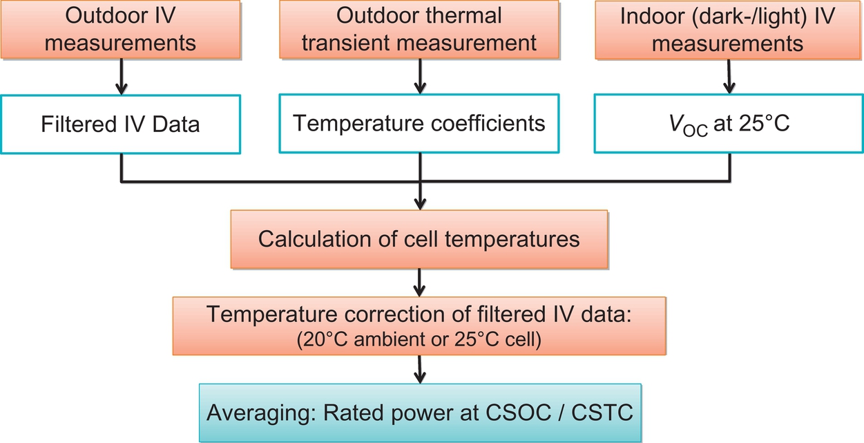
The outdoor I–V measurement of CPV modules provides a dataset of I–V curves measured at various prevailing ambient conditions. This I–V dataset is translated to CSOC and CSTC in two steps: filtering and temperature correction.
The filtering step removes all I–V curves measured at prevailing ambient conditions which are not stable and differ too much from the standard conditions. Therefore, a dataset of I–V curves is required which include datasets fulfilling the filtering criteria. For the step of temperature correction, the representative temperature for the cells inside the module is required. This representative cell temperature is calculated using module temperature coefficients and the module open-circuit voltage (VOC) at 25°C. The temperature coefficients are determined from TTM. The VOC at 25°C is calculated from indoor I–V measurements. In the following the rating procedure is described in more detail.
The basis of the CPV module power rating is the measurement of I–V curves outdoors in a test period comprising varying prevailing ambient conditions. The module is mounted and aligned on a sun-tracking unit while its I–V curves and the ambient conditions are recorded automatically. The ambient conditions have to be recorded in an interval of less than 1 min and the duration of the I–V sweep should be less than 15 s. The I–V dataset shall include at least three separate SMR crossing points. The SMR values change during one day due to atmospheric composition and due to air mass (AM). SMR values of unity indicate standard spectral conditions. An SMR crossing point is reached when the SMR values get close enough to unity to fulfil the filtering criteria. The I–V dataset is filtered for stable conditions and for ambient conditions similar to CSOC. The most important criteria are as follows:
(i) DNI shall not vary more than 10% in 10 min before the I–V sweep and not by more than 1% directly before and after the I–V sweep.
(ii) The portion of DNI from global normal irradiance shall be above 80%.
(iii) All SMR values shall be within unity by ± 3.0%.
The first criteria shall assure that the cell and lens temperatures are stable. The second criteria assures a clear sky and the third one permits only prevailing spectral conditions close to the AM1.5d reference conditions. Especially the SMR filtering criteria is a trade-off between effort and accuracy. A tighter filtering around unity will decrease the measurement uncertainty, whereas a wider filtering increases the amount of days throughout the year where test labs can fulfill the filtering criteria and thus reduces the length of the test period.
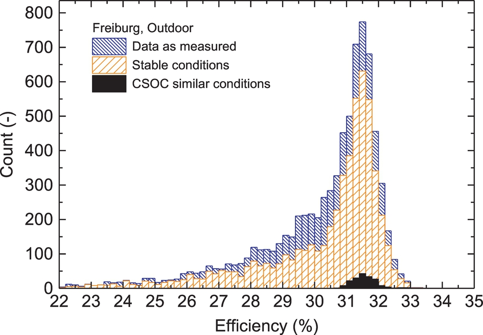
Fig.10.12 shows an example of the module efficiency histogram of I–V curves measured at a FLATCON-type CPV module at Fraunhofer ISE within one full year of operation. Additionally, Fig. 10.12 shows the distribution of module efficiency after applying the filter criteria for stable conditions and for CSOC similar conditions. The remaining dataset of module efficiencies is used to calculate the CSOC and CSTC power outputs after applying a temperature correction.
The temperature correction of the module efficiency is done using module temperature coefficients and a representative cell temperature. The temperature coefficients are obtained by TTMs. TTM means mounting and aligning a CPV module on a sun-tracking unit. Cover the module and wait until it is close to ambient temperature. Measure the module back-plate temperature. Then uncover the module and measure I–V curves while the cells in the module are heating up. The heating process commonly takes around 10–20 min and the back-plate temperature is increased by 10–20 K in this time. Fig. 10.13 shows the VOC, ISC/DNI, FF and efficiency as a function of back-plate temperature derived from TTM. For the outcome of the TTM it is important that the back-plate temperature is changing in a one-to-one rate with the cell temperature. This one-to-one rate is given if deviations from linear correlation of VOC versus back-plate temperature are small. In the first seconds after uncovering the module such a one-to-one rate is typically not found and this data has to be discarded. The temperature coefficients for VOC, ISC, FF and efficiency are then obtained by linear fits to the TTM data as shown in Fig. 10.13. The temperature of the cell in the module is typically higher than the back-plate temperature of the module. Thus, TTM can only provide relative temperature coefficients. The absolute temperature of the cells is calculated using the module VOC at 25°C. The difference of the VOC at increased cell temperature to the VOC at 25°C in combination with the relative temperature coefficient of the VOC gives the absolute cell temperature. This calculation of cell temperature is based on the one-diode model and described in Ref. [21].

The module VOC at 25°C is derived from I–V curves measured indoors. There are two options for measuring the required I–V curves. First, measuring the module dark I–V curve and second using a sun simulator for CPV modules to measure the light I–V curve. In both cases the module I–V curve is measured at 25°C room temperature.
The advantage of the dark I–V option is that a CPV module sun simulator is not required. In this case, the dark I–V of the CPV module is measured at 25°C room temperature. The dark I–V curve needs to be corrected for series resistance as explained in Ref. [21]. The module VOC at 25°C corresponds to the voltage of the corrected dark I–V curve where the current equals the module ISC.
Extracting the VOC from the sun simulator light I–V curve requires setting up the intensity of the sun simulator. For this reason, the module ISC is derived from outdoor I–V measurements and translated to 25°C cell temperature using the module temperature coefficients. The intensity of the sun simulator is varied until the measured module ISC indoor matches the outdoor ISC. Then the module light I–V curve is measured and the VOC at 25°C is derived from this I–V curve.
One may ask at this point why the CPV module sun simulator is not used to determine the power output at CSTC? In this case the translation of outdoor I–V data to 25°C cell temperature would not be necessary. The answer to this question is the significantly higher uncertainty of the currently available sun simulators compared to outdoor measurement.
Finally, Fig. 10.14 shows the histogram of module efficiency values derived at CSOC after applying the temperature correction to 20°C ambient temperature and at CSTC after translating the CSOC efficiencies to 25°C cell temperature. The rated efficiencies are determined as the average values of the efficiency distribution, ie, 31.7 ± 0.5% for CSOC and 34.3 ± 0.5% for CSTC. The rated power at CSOC is the rated CSOC efficiency times a DNI of 900 W/m2 and multiplied by the lens aperture of the CPV module, whereas the rated power at CSTC is the rated CSTC efficiency times a DNI of 1000 W/m2 and multiplied by the lens aperture of the CPV module.

10.4 System performance and energy yield prediction
The objective of this section is threefold: Firstly, we focus on measuring the actual power output of CPV systems and power plants and on recording the prevailing meteorological conditions. Secondly, we quantify the performance of CPV systems by calculating two performance indicators, performance ratio and performance index, which includes comparing the actual measured power output and the expected output from a performance model. Thirdly, we present some frequently used software tools for modelling the prospective power output and the typically involved loss mechanisms. A large part of this section is based on documents of the IEC, namely IEC 61724-1 (‘PV System Performance—Part 1: Monitoring’) and IEC 62670-2 (‘CPV Performance Testing—Part 2: Energy Measurement’).
10.4.1 Actual energy output and prevailing meteorological conditions
In a first step, monitoring of the actual performance of a CPV plant requires the installation and maintenance of a data acquisition system. CPV plants are usually equipped with SCADA (‘Supervisory Control And Data Acquisition’) systems which include data loggers and sensors for the measurement of electrical and meteorological parameters. IEC 61724-1 classifies such measurement set-ups into three categories, depending on whether the sampling rate and the precision of the sensors is considered to be high (Class A), medium (Class B) or low (Class C). These classes may coincide with usage at utility (Class A), commercial (Class B) and residential (Class C) installations. As most CPV plants are built at the utility scale, we may assume that data collection fulfills the Class A criteria, ie, data recording at 1-min intervals, 3% or less uncertainty for the measurement of the DNI, 2% or less uncertainty for DC power and utility-grade AC energy meters. Another relevant document, IEC 62670-2, requires that the measurement system be calibrated and checked for linearity, stability and correctly working integration before data acquisition starts. While electrical meters are installed in protected enclosures and require little maintenance except for occasional checks of the calibration, measurement of the DNI requires significant attention and efforts to ensure high data quality. By their measurement principle, pyrheliometers are exposed to outdoor conditions including dust and rain and require precise alignment and mechanical tracking, regular cleaning of the aperture and regular recalibration. As the uncertainty of the irradiance data often dominates the overall uncertainty of the derived performance indicators, it is strongly recommended to use high-accuracy pyrheliometers and implement a strict cleaning schedule with minimum weekly cleaning of the aperture and documentation of each cleaning event in a logbook.
In a second step, automated and manual quality checks should be applied and questionable data be flagged and filtered, before data is summed to obtain hourly, daily, weekly, monthly and yearly values. IEC 61724-1 lists a number of quality checks, including applying physically reasonable minimum and maximum limits, maximum rates of change and comparing measurements from multiple sensors. Logbooks should be inspected particularly for periods of insufficient pyrheliometer cleaning or delayed recalibration. Periods during which data is omitted from summation or further analysis due to low quality need to be treated with special care, as pointed out in the section on data postprocessing rules of IEC 62670-2. As summed data may be used for the calculation of performance indicators in a later step, it is of high importance to symmetrically exclude periods during a gap that occurred either in the irradiance or power time-series, or in both, in order to avoid misleading results when ratios of electrical and irradiance energy are calculated.
10.4.2 Performance ratio and performance index
Performance ratio and performance index are standardized indicators defined consistently for nonconcentrator and concentrator PVs [22]. Performance ratio, as defined for nonconcentrator systems in IEC 61724-1 and for concentrator systems in IEC 62670-2, is a measure expressed in percent, for the overall effect of losses on the power output of a plant. As shown in Eq. (10.4), it is defined as the ratio of the final AC yield Yf,AC (Eq. 10.5) and the reference yield Yr (Eq. 10.6). This is equivalent to the product of (100% − Li) of i losses. The Li losses could be shading loss, soiling loss, cell temperature loss, etc. EAC is the AC energy and PCSTC is the plant DC power at CSTC. CSTC stands for ‘Concentrator Standard Test Conditions’ as per IEC 62670-1, ie, 1000 W/m2 DNI, 25°C cell temperature and direct normal AM1.5 spectrum. EDNI is DNI energy.


Performance ratio can be regarded as a normalization of the generated AC energy by a ‘rough estimate’ [23] of the expected energy, namely by name-plate power PCSTC and DNI (ie, EDNI). As loss factors, such as temperature or spectral losses, are not considered in this normalization, performance ratio is below 100% even for a well-functioning plant, which makes it hard to interpret.
When calculating performance index, in contrast, we compare the measured energy output of a power plant to the energy output calculated with a potentially quite complex model. As such models try to accurately consider various loss factors, performance index actually reaches 100% once the plant delivers the amount of energy that is expected from the simulations. In IEC 61724-1, performance index is defined as the ratio of the measured AC energy to the expected AC energy (Eq. 10.7).
As pointed out by Mokri and Cunningham [23], ‘deviations from 100% [performance index] can be caused by many factors, including errors or incorrect assumptions during design, poor installation workmanship, equipment failure or degradation, etc.’ Diligent analysis may be required to understand the root cause of deviations from 100%, as it may also be the case that the plant works well, but the model may not be precise enough or the meteorological data fed to the model may be compromised.
10.4.3 Typical loss mechanisms and models to estimate the prospective energy output
In Fig. 10.15 we compare the actual (columns) and the modelled (dashed and solid lines) monthly performance ratio of a CPV plant installed in South Africa. The plant is installed at a site with notable temperature differences between summer and winter, as reflected in the monthly DNI-weighted ambient temperature (black crosses) defined in (Eq. 10.8). The modelled performance ratio values plotted as a dashed line stem from performance Model A which does not include typical CPV-specific loss mechanisms. In contrast, Model B (results plotted as dashed line) includes such mechanisms. Obviously, Model B captures the observed seasonality of the performance ratio much better than Model A, so it is worth having a closer look at typical CPV-specific loss mechanisms in the next paragraphs.


Temperature dependence of the optics: The efficiency of concentrating optical elements used in CPV modules may show a nonnegligible dependence on the temperature of the optics (Toptics), and indirectly on ambient temperature (Tambient). The temperature dependence of the refractive index and different coefficients of thermal expansion of composite materials, such as silicone-on-glass, may contribute to a temperature-dependent internal misalignment of CPV modules, as described by Kurtz et al. [24]. For example, the performance ratio simulated with Model B in Fig. 10.15 includes a simple linear model to approximate the loss due to the temperature dependence of the optics, similar to the model shown in Eqs (10.9), (10.10). Model B thereby captures the lower performance during cold winter months (May–September), while Model A (which does not consider this loss) even predicts higher performance during winter than during summer, as cell temperature losses are reduced with decreasing temperature. Assuming that an arbitrary CPV module would be designed for best internal alignment at a temperature of the optics of 30°C, (Eq. 10.9) could describe a linear model for the loss due to nonoptimal temperature with parameter ![]() for
for ![]() and
and ![]() for
for ![]() .
.
The temperature of the optics could be estimated from ambient temperature and wind velocity with (Eq. 10.10) and parameters like ![]() and
and ![]() .
.
The values given in this example are arbitrary and have to be derived for specific CPV module designs from indoor or outdoor measurements of representative samples, such as described by Faiman et al. [25]. Based on such experimental data it also has to be carefully verified if the simplified Eqs (10.9), (10.10) approximate the observed module behaviour with sufficient accuracy. In a more detailed approach, Steiner et al. [18] used finite element and ray tracing methods to consider the temperature sensitivity of the optics in their ‘YieldOpt’ model.
Spectrum: Multijunction solar cells are inherently sensitive to the spectrum of the light due to the serial interconnection of several subcells. The subcell which produces the lowest current limits the overall current of the multijunction cell. The spectrum of the light impinging on the solar cells depends on geographical and meteorological parameters such as geometrical AM and haziness of the atmosphere, as well as on the spectral transmission of the optics. As for the temperature sensitivity of the optics, the underlying mechanisms of the spectral loss are complex and need to be modelled with an adequate level of simplification. Strong simplification is applied in the linear AM model of PVsyst [26] and in the parabolic model of Strobach et al. [27]; both do not consider atmospheric parameters. In contrast, Steiner et al. [18] rely on measurements of multifilter rotating shadowband radiometers to obtain atmospheric parameters and modify the clear-sky DNI spectrum accordingly using the SMARTS model.
Cell temperature: Temperature distribution across CPV modules and solar cells is usually nonhomogeneous due to the principle of point-focusing the irradiance. In the technology development phase, heat transfer models may be required to estimate and optimize cell temperature based on conduction, convection and radiation processes. However, linear temperature coefficients, experimentally determined as per IEC 62670-3 or as in the previous chapter, are usually sufficiently precise for modelling the field performance of CPV systems. If measurements of the open-circuit voltage, which serves as a surrogate for cell temperature, are not available, cell temperature may be estimated with heat transfer models from ambient temperature, irradiance and wind velocity, as implemented in PVsyst and NREL SAM [28,29].
Module I–V-characteristics: Electrical models for the voltage–current characteristics of nonconcentrator and concentrator modules may either predict the full I–V curve (‘equivalent circuit models’) or predict only the characteristic points of the I–V curve, such as Impp, Vmpp, Isc, Voc (‘point-value models’) [30]. Some examples for equivalent circuit models include the one-diode model implemented in PVsyst [28], the ‘five parameter single-diode model’ available in the SAM package by NREL [31] and the Spice network model by Steiner et al. [18]. The most widely used point-value model is the Sandia PV Array Performance Model [29], which can also be chosen in the SAM package.
Shading: Modelling the shading loss of CPV systems follows the same principles as for nonconcentrator systems, but may have to consider more complex geometries due to widespread use of two-axis trackers. The solar irradiance that does not reach the CPV modules due to shading cannot be converted to electrical energy and needs to be considered as so-called ‘geometrical shading loss’, often estimated by applying surface projection and intersection processing on a three-dimensional model of the plant [32]. Depending on the internal wiring of cells and modules in series and parallel strings, the usage of bypass diodes and the shape of the shadows, an additional ‘electrical shading loss’ needs to be taken into account [33]. It is caused by different current–voltage characteristics of unshaded and partially shaded CPV modules that are connected to the same maximum power point tracker of an inverter. The inverter chooses a common load resistance for all modules, resulting in an electrical shading loss due to nonoptimal power extraction from some modules.
Soiling: Deposition of dirt particles on the surface of CPV modules leads to soiling losses, which may be considered as a constant loss of a few percentage points in a first approximation. More detailed models should consider site characteristics such as soil type and vegetation, frequency of rainfall, wind velocity and direction. Based on a daily soiling rate, a cleaning threshold and a grace period after cleaning, Kimber et al. [34] empirically derived a soiling model. Winter et al. showed that small rain events may significantly reduce soiling loss [35].
Tracker pointing error: The acceptance angle under which incoming sunlight reaches the solar cells inside the CPV modules is limited due to the usage of concentrating optics and cost-efficient designs. The sensitivity of the module power output on misalignment can be characterized using a procedure described in IEC 62670-3, resulting in an ‘acceptance angle curve’ that relates misalignment in units of degrees to power loss in units of percent. The pointing accuracy of CPV trackers is limited and can be quantified with a method described in IEC 62817, resulting in a frequency distribution of the pointing error in units of degrees. The loss due to tracker pointing error for a specific combination of CPV modules and trackers can be estimated by combining the results of both aforementioned procedures.
Tracker wind stow: Two-axis trackers may only operate in tracking mode up to a maximum wind velocity vwind,max which depends on the design of the tracker and its foundation. SCADA systems continuously measure wind velocity and, when vwind,max is exceeded, automatically steer the trackers to a safety position in which the tracked plane is parallel to the ground. If this happens during sunny periods, the resulting loss is 100%, as the modules are no longer aligned with the sun. The loss for longer periods may be estimated by processing a time-series of wind velocity and DNI, replacing the DNI values with 0 during high wind velocity periods and calculating the effectively captured DNI. As wind velocity is a dynamic quantity, it is recommended to use a time-series with a step size of 5 min or less. The time required to move from tracking mode to the safety position and back, as well as hysteresis times of the SCADA systems should be considered in the model.
DC to AC conversion: Inverters used with CPV systems can be modelled in almost all aspects similar to inverters connected to nonconcentrator systems, eg, using the Sandia inverter model [36]. However, there is one point that requires particular attention: As DNI may change much faster than global irradiance, a slowly responding inverter may not be able to follow steep DNI and DC power ramps, leading to so-called ‘switch-on loss’. If inverters with short delay times and fast ramping capability are chosen, the switch-on loss becomes negligible. For slowly responding inverters, the switch-on loss can be estimated based on the actual delay times and ramp rates and a DNI time-series with high time resolution (1 min or less).
Parasitic consumption: As CPV power plants usually contain more moving parts than nonconcentrator plants, such as trackers and possibly active ventilation or cooling systems, they usually show a higher loss due to parasitic consumption for powering motors and control boards. Manufacturers often provide typical consumption values on data sheets. Procedures for verifying parasitic consumption data are described in IEC 62670-2.
Frequently used modelling tools:
• The PVsyst software (http://www.pvsyst.com) is not only widely used for nonconcentrator plants, but considers also specific loss factors of CPV by a step-wise linear model for the temperature dependency of the optics and the spectral dependency of the multijunction cells, referred to as ‘Utilization Factor’ [37]. PVsyst's shading model is rather user friendly and can handle complex geometries of several hundred CPV trackers. The module IV characteristics can either be based on the one-diode model by Duffie and Beckman [38] or Sandia's Array Performance Model [29]. PVsyst offers an extensive graphical user interface, but lacks support for a scripting language. Although the documentation is extensive, some algorithms and details of the PVsyst software remain undisclosed.
• In contrast to PVsyst, the PV_LIB toolbox (https://pvpmc.sandia.gov and https://github.com/pvlib/pvlib-python), initiated by Sandia and extended by various contributors, provides full transparency of its algorithms, as they are disclosed under the Berkeley Software Distribution (BSD) license and can be easily extended with new functionalities. Being a collection of scripts that includes module and inverter models, data handling functions and atmospheric and irradiance models written in Matlab and the Python programming language, this toolbox targets engineers and modellers with programming skills and does not offer a graphical user interface.
• The SAM software (https://sam.nrel.gov) developed by NREL presents a mixture of the concepts used by PVsyst and the PV_LIB toolbox. On the one hand, it presents user friendly graphical guidance through typical simulation tasks (which also include renewable sources other than PVs, and financial modelling) and on the other hand, it includes scripting language support and a software developer kit so that users can extend the functionalities.
10.5 Future trends
CPV technology has made great technological progress during recent years. The highest ever reported efficiencies for PV cell and module of 46% and 38.9%, respectively, were achieved by this technology. Obviously, one can name this technology the ‘high end’ of all PV technologies. While the technology had progressed extremely fast, the market is still in an infancy status. Only very recently have larger installations of 40-100 MWp size been installed in the field. The cumulative production volume of CPV (LCPV and HCPV) technology is below 400 MWp. If compared with flat-plate technology, which is beyond 200 GW, it is obvious that the contribution to the PV market is currently negligible. In other words, marketwise CPV technology is on the same level as flat-plate technology was in the year 1993. However, the costs of the CPV technology are much lower than the cost of flat-plate technology at that time. Therefore, the cost of CPV is promising and the current challenge for CPV technology is to install many more MWs, thus growing the market and benefitting from manufacturing scaling effects. According to the price-experience curves known for other technologies, this will lead to a fast reduction in costs of CPV systems. On the other hand, the performance of CPV still has room for further improvements. Cell efficiencies beyond 50% and module efficiencies of 42% are in reach (see Fig. 10.7). It is important to note that the transfer from R&D results obtained in laboratories into industrial products has turned out to be extremely fast in CPV technology. For example, reported record cell efficiencies from laboratories are commercially available 3 years later.
For the future of CPV technology it is also important to proceed with the development of IEC standards. Standardization has turned out to be very important for market development. Standards help to establish trust in the products of the supplier and pave the way for financing. Currently several IEC standards are under preparation. As detailed in this chapter, some of the standards are very advanced and could be already used, but they are not yet finalized.
Further information on the technology and market of CPV technology can be found in the proceedings of the International Conference on Photovoltaics, which are published in an AIP series. The recent proceedings of CVP-10 till CPV-12 are accessible via open access and can be found here: http://www.cpv-12.org/proceedings.html.
Interested readers are referred to books about CPV technology; see reference list [39,40].