Photovoltaic module stability and reliability
D. Jordan; S. Kurtz National Renewable Energy Laboratory (NREL), Golden, CO, United States
Abstract
Profits realized from investment in photovoltaic will benefit from decades of reliable operation. Service life prediction through accelerated tests is only possible if indoor tests duplicate power loss and failure modes observed in fielded systems. Therefore, detailing and quantifying power loss and failure modes is imperative. In the first section, we examine recent trends in degradation rates, the gradual power loss observed for different technologies, climates and other significant factors. In the second section, we provide a summary of the most commonly observed failure modes in fielded systems.
Keywords
Reliability; Durability; Degradation rates; Failures; Field test; Aging
Acknowledgement
This work was completed under contract no. DE-AC36-99GO10337 with the US Department of Energy.
3.1 Introduction
As the installed capacity of the photovoltaic (PV) industry is approaching 200 GW, investors seek confidence in long-term PV performance. Profitable investment in PV will benefit from decades of reliable operation. The discipline of reliability has been well established and has led to significant quality increases for many types of products, including PV systems; however, the application to PV modules is challenging for several reasons. The desired long lifetime prevents direct verification, especially because of the short product development life cycle. In addition, the size and cost of PV modules typically inhibits testing of a large number of samples. Furthermore, PV modules are complex and can display a variety of failure modes. Because of the synergistic nature of the different failure modes an understanding of the underlying physical and chemical processes is essential. Finally, the use environment can be highly variable, leading to a climate dependency of different failure modes. As the industry enhances service life prediction, improved accelerated lifetime tests need to be developed. For years the industry relied on extending the qualification testing of IEC 61215 and IEC 61646 to establish confidence in its products [1]. Arbitrary extension of accelerated tests, however, may not lead to the desired result, as failure modes observed in accelerated testing should match the ones observed in the field. Therefore, detailing and quantifying failure modes and power loss from field observation is an essential part of developing lifetime service tests. The first part of this chapter is dedicated to the lifetime and gradual power decline and the second part to the various failure modes that have been documented.
3.2 Module stability and lifetime
3.2.1 Historical survey
As modules and balance-of-system components of a PV system age, they gradually lose some performance. Most commonly, PV module manufacturers guarantee against this loss by promising 80% of nameplate power after 25 years whether in a stepped or linear fashion. The decline is expressed in relative percentage, such that a module with a hypothetical absolute efficiency of 20% today would decline to 17.5% after 25 years at an annualized (relative) rate of 0.5%/year, assuming the decline is approximately linear. The decline or degradation rate has significant financial consequences, as this rate directly affects the yield and, therefore, the cash flow in future years. In financial projections, the value of a PV project after 25 years is often assumed to be negligible, yet our simple hypothetical example illustrates that such a module would present a considerable residual value after 25 years. At the time of this writing, more than 30 studies of systems older than 20 years have been reported, with some at 30 years and one even approaching 40 years. As such, there appears to be no end to the lifetime of certain PV systems. Yet other reports exist of premature decline due to manufacturing defects or poor installation quality.
For an investor, this presents a considerable quandary associated with financial risk. Therefore, it is important to understand, detail and quantify the various factors influencing the performance loss curves. Some of the authors first aggregated and analysed the public knowledge of PV lifetime measurements, which were later reanalysed [2,3]. As can be seen in the colour-coded map (A) and in the graph of studies exceeding 20 years (B) of Fig. 3.1, this topic has seen an increased interest in recent years. This chapter offers an updated analysis with a goal of providing better answers to some of the questions that remain open.

More than 11,000 annual degradation rates have been aggregated and analysed in this section. The first observation in the histogram of Fig. 3.2A of all data (solid blue) is that the distribution is bimodal, a peculiar property that needs further discussion.

As the degradation rates are impacted by a variety of factors, including (but not limited to) manufacturer, model, technology, climate, mounting, failure modes, measurement uncertainty, etc., it is important to delineate the factor causing the bimodality. Next to these hardware-related variables influencing the long-term performance assessments, statistical procedures including (but not limited to) methodology and sampling can also influence the determined rates and therefore the overall distribution. To accurately assess the status and the health of the industry in general, a representative sample is essential. As the present study is not based on a designed study but a correlational study, it is important to investigate the aggregated values in different ways to ensure the absence of unintended bias. To illustrate this, we consider this hypothetical example: 10 studies investigating the long-term performance of 10 different modules, in different climates, mounting configurations, etc., analysed together with one additional study investigating a single product, in a single location but investigating 100 modules. The aggregated distribution would be dominated by the single study but might not be representative of the product population in general. Thus, to reduce sampling bias, that is, the over- or under-representation of a group, we present the data aggregated from the literature both by including all reported measurements and by using the median of each study and system. However, even this method may not be the best methodology to find a representative sample. Consider again a hypothetical example of two studies: One study examines 10 products at high accuracy and a similar study assesses an equal number of products at very low accuracy. By using the median of each study, the sampling bias is superficially reduced but this method would equally weigh each study. However, one would probably choose to give the more accurate study more weight than the less accurate study.
Therefore, we also show a degradation rate distribution of studies that we consider to be high quality based on the following criteria: multiple measurements were taken for increased confidence; the measurement methods and calibrations were clearly described and are generally similar at each measurement point; details on the installation (disregarding proprietary considerations) are provided. Each of these analytical methodologies is imperfect, but it is interesting to note that they consistently lead to a unimodal distribution centered in the 0.5–0.8%/year range. Furthermore, the aggregation of degradation rates through survey of published information may induce sampling bias because modules or systems at high decline rates may be less likely to remain exposed in the field than those with smaller decline rates. In contrast, some studies may examine prototypes and not commercially available products without specifying. Finally, every effort was made to separate light-induced degradation (LID) from long-term performance decline. LID is a short-term performance degradation upon initial light exposure because of light-induced chemical reactions that increase the effects of defects in the semiconductor material.
Nevertheless, since we are largely limited to reporting the information provided, LID artefacts cannot be completely excluded, especially when considering data collected on thin-film technologies.
3.2.2 Nameplate rating
Many studies were found to have utilized only the nameplate rating and one measurement to determine a degradation rate slope. One-measurement studies often are a result of missing beginning-of-life measurements because they were (1) never taken or (2) because of the long life of the PV system, they can no longer be recovered. To assess the durability of the module or system, the analyst has no choice but to compare the measurement to the nameplate rating. Several implicit assumptions are made in this procedure:
1. The nameplate rating was accurate at the beginning of the PV life.
2. If an ensemble of modules is measured, the ensemble of performance starts as a point source and not as a distribution with a shape defined by a convolution of the binning practices of the manufacturer and the process control. Modules are sorted according to their measured power and allocated to specific rated power products, ‘bins’; therefore, as an example, modules from a nominal 250 W ‘bin’ may produce slightly more or less power depending on the specific manufacturer's sorting practices. Furthermore, nameplate rating constitutes a measurement by itself and several papers have discussed the uncertainties involved with the rating measurements [4–6]. The combination of these effects leads to the product tolerance, which has changed significantly over the past several decades.
3. Beginning-of-life LID is not considered consistently. For crystalline silicon (x-Si) this occurs on a short time scale but for some thin-film products the stabilization process may take from several months to years but is often included in the manufacturer's rating [7].
The difficulty is to take these effects into account to accurately assess PV durability, yet in many durability studies these uncertainties are often not discussed. To better gauge the uncertainty associated with one-measurement studies, Fig. 3.3 shows an extensive (yet most likely not comprehensive) graph on the history of module measurements with respect to their nameplate rating [8–19]. Indoor I–V measurements are indicated by red open circles and outdoor I–V data by blue open triangles. As a guide to the eye, a 10% discount line is also shown. Considerable spread exists but it appears that measurements on solar simulators tend to be closer to the nominal nameplate rating. However, the data points only go back to the mid-1990s. With the exception of a few data points in 2011, the outdoor measurements trend closer towards the nameplate rating in recent years, an effect which may be attributable to the change in manufacturers’ tolerance. At the time of the writing, most PV module manufacturers warrant tolerances of 0% to positive deviations, whereas older modules often carried equally symmetric positive/negative deviations. As discussed in the previous section, another reason for the larger outdoor deviation may be associated with the confounding effects of measurements and soiling.

In addition LID is often contained in these data points. However, it must be emphasized that, for long-term performance, LID must also be taken into account. The 2011 study in Fig. 3.3 includes modules that had been on sun for more than 1 year; thus these modules may not truly represent beginning-of-life measurements, a fact that may explain some of the low-lying outliers. It is evident from Fig. 3.3, even if the graph is not comprehensive, that considerable deviations at the beginning of life may be expected, depending on the specific production time and tolerances. Therefore, depending on the fielded time and the specific modules, degradation calculations may be significantly impacted. These considerations should be included in an uncertainty budget. Additionally, for these reasons, one-measurement studies, which depended upon nameplate ratings, were not included in the high quality data set category in Fig. 3.2.
3.2.3 Technology trends
In this section we examine the aggregated degradation rates by technology and the evolution over the past decades. Fig. 3.4 is colour-coded by the different technologies. Multicrystalline (multi-Si) and monocrystalline (mono-Si) have been combined into one category as a significant number of studies specify x-Si but do not disclose any other details. The type of study or measurements is symbol-coded. Degradation of 1%/year and 0.5%/year are indicated by red solid and dashed lines, respectively. Each technology category is partitioned into the decade of installation wherever possible. Because of considerable data variation, boxplots representing the interquartile range and the median are overlaid over the data points.
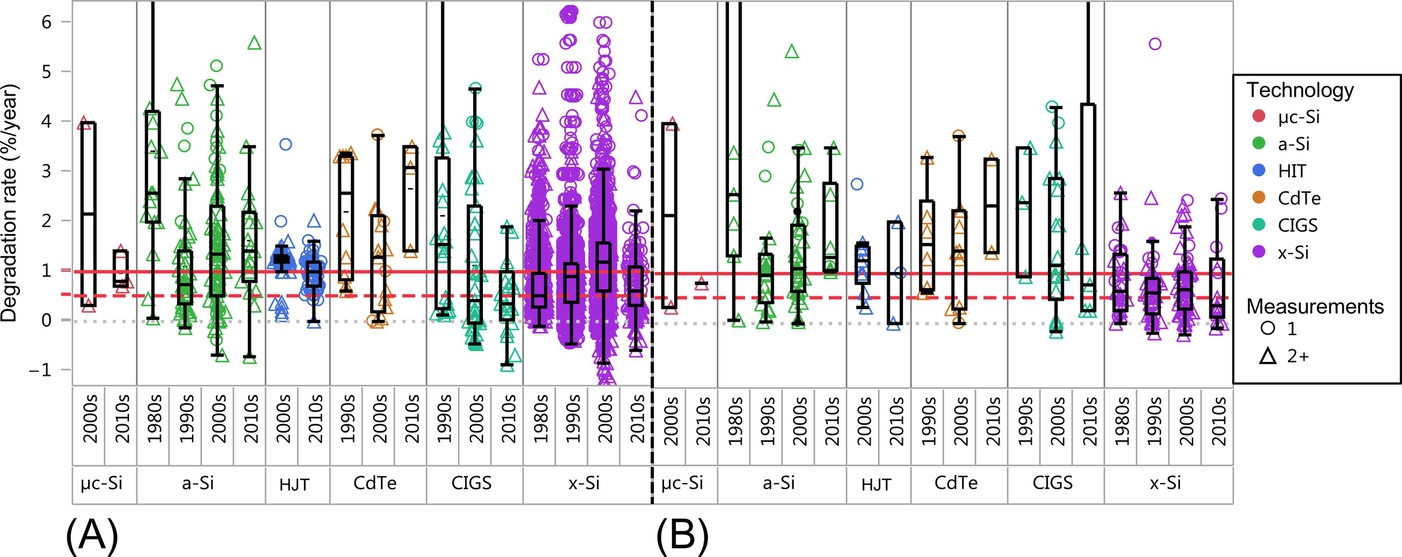
Microcrystalline (μc-Si) is a relatively new technology; therefore, long-term performance assessments are relatively scarce yet tend to aggregate around 1%/year. In contrast, amorphous silicon (a-Si) has a history almost as long as x-Si technologies. The technology initially suffered from high degradation, and then significantly reduced degradation before an increase to above 1%/year that appears to be consistent in the past 15 years. Sufficient data are available to partition the heterojunction technology (HJT) into its own category. Similarly to μc-Si, the HIT technology is not that old; only two subcategories are available with a median degradation that appears to be consistent around 1%/year. Cadmium telluride (CdTe) shows behaviour similar to a-Si as a significant decline in degradation occurs from the first to the second decade, followed by an increase in the third decade. This increased degradation rate may be influenced by one-measurement studies and longer stabilization for some products [7]. After suffering from high initial degradation followed by the first reports of low degradation, copper indium gallium selenide (CIGS) appears to have settled for a median of around 0.5%/year.
The x-Si is the largest category and shows initial degradation of around 0.5%/year in the first decade. In subsequent decades the degradation appears to increase to slightly above 1%/year before receding to 0.5%/year in the current decade. Many of the data points in the 1990–2000 decade that showed an increase in degradation were measured using the nameplate rating. In addition, as we discussed previously, sampling bias is a serious concern. Thus, Fig. 3.4B shows the same data but uses the median of each study or system. It can be seen that most categories appear unchanged and the conclusions we stated previously are the same. Considerable change, however, can be seen in the x-Si category. The median degradation for x-Si technologies now appears to be consistently around 0.5%/year, illustrating that the higher rates reported in Fig. 3.4 for x-Si may reflect a small number of studies that reported data for thousands of modules. The mean (not shown in Fig. 3.4) for x-Si dropped from 0.99%/year for the 1980s to 0.72%/year, then was 0.78%/year and 0.77%/year for the 1990s, 2000s and 2010s, respectively.
3.2.4 Climate and mounting
Recent studies describe higher degradation rates in hotter climates compared to more moderate climates [20–23], which are also reflected in the guidance provided by module manufacturers [24]. Degradation rates are influenced not only by temperature but other factors such as age, measurement uncertainties, methodologies, technology, product type and mounting. It is of considerable interest whether the aggregated data can corroborate these findings.
To avoid the confounding technology effect, Fig. 3.5 shows x-Si degradation rates (A) and the median for each study and system (B) partitioned by the number of measurements and climate zones. The climate zones are based on the Köppen–Geiger classification but aggregated into four simplified categories [25]. Statistical analysis revealed significantly higher degradation rates for studies using the nameplate rating. In addition, hotter climates show a trend towards elevated degradation rates compared to cooler climates. Mounting configuration—roof- versus rack-mounting—leading to prolonged elevated temperatures may also lead to increased degradation [23,26,27].

3.2.5 Module versus system degradation
Very few studies exist where module and system performance data are investigated at the same time and thus it is not clear how module long-term performance relates to system performance. In Fig. 3.6 we partition crystalline silicon (x-Si) high-quality data into system and module data. Cumulative distribution functions for all data (solid lines) and median values per study and system (dashed lines) are shown. The number of data points is again given in brackets. The cumulative probability median is indicated by a dashed horizontal line, whereas the 0.5%/year and 1%/year degradation are indicated as vertical dashed and dash-dotted lines, respectively. At the cumulative probability median, the system curves are very similar around 0.6%/year. The degradation rates for the module data are below the systems data and show some difference depending on whether all data or median per study and system are shown, which may enable us to infer some uncertainty associated with this comparison. It follows that one would expect system degradation to be similar or slightly larger than module degradation at the median. Module and system curves start to deviate more substantially for worse-performing products. This may be consistent with a recent more detailed examination of a 20-year-old x-Si system, in which it was found that the worst-performing module was limiting the string, and, in turn, the worst-performing string was limiting the system [8]. If the modules in a given system degrade similarly, the system will degrade close to the median module; conversely, if the modules show substantial spread in their degradation behaviour, the system degradation may be significantly different from the median module behaviour.

3.2.6 Nonlinearities
The first challenge in long-term performance prediction is the question of linearity. Many PV technologies, especially thin-film technologies, exhibit nonlinearities at the beginning of their useful life. The initial rapid decline for amorphous silicon (a-Si) has been well documented [28]. The initial rapid decline occurs during several months before the onset of the long-term trend, as shown in Fig. 3.7. Some CdTe products show a similar behaviour [7]. The CIGS system shown in Fig. 3.7 shows a distinctly different behaviour; an initial increase during the first several months of light exposure is followed by the onset of the long-term degradation. It is evident from these examples that the initial trend is different from the long-term behaviour. In addition, if the initial phase is included in the evaluation, the long-term prediction would include a substantial, yet unintended bias.

In addition to the beginning-of-life phase, the wear-out phase in the lifecycle of PV modules can include nonlinearities. Fig. 3.8 displays four studies examining an ensemble of modules several times during the life of a PV system, each system having been fielded for at least 20 years. The sample from the Colorado, USA study is too small to confidentially establish linearity [8]. The California, USA study shows a fairly linear behaviour for the central tendency of the modules [29]. However, the worse-performing modules display distinct signs of nonlinearity. Similar trends can be observed in the studies from Switzerland [18] and Italy [30] of modules that were exposed for 30 years.

3.2.7 Financial impact
On the systems level, several studies have emerged recently that partition continuous data into shorter time intervals allowing the determination of several subsequent degradation rates instead of one overall degradation rate [31,32]. This is a promising trend, as it allows delineating the properties of the degradation curve and provides more information than one overall degradation rate. Quantifying nonlinearity of degradation curves, in contrast to rates that imply linearity, can have significant impact on financial aspects of a PV project, such as the levelized cost of energy (LCOE) [33]. In summary, we may conclude that nonlinear behaviour may depend on a variety of factors, such as technology, product, climate, system load, etc., as some products will be more susceptible than others.
3.2.8 Other factors
Finally, the load under which a PV module or system is exposed may also influence the overall degradation. Crystalline Si modules were shown to have a significantly higher degradation after 20 years of field exposure when they were grid-connected through an inverter compared to open-circuit condition [34]. In contrast, for a-Si technology open-circuit conditions led to significantly higher degradation compared to under continuous load [35].
3.3 Reliability and failure modes
3.3.1 Historical survey
Service lifetime prediction, as discussed in Section 3.1, depends on developing accelerated tests that can duplicate failure modes from field observation. Information on field failure modes can be obtained empirically through site visits [36], warranty returns [37] and/or maintenance records [38]. Recently the International Energy Agency PV Power Systems Program—Task 13 published a detailed review on failures of PV modules based on literature and site visits [39]. The treatise discusses at length inspection tools, observed failures observed and new proposed test methodologies. Different failure modes are classified by safety and their different time series behaviour, eg, linear versus nonlinear. In practice it is often difficult to distinguish between different time series behaviour and estimating the impact of a failure mode for several reasons. Different products may be susceptible to different failure modes at different times in their life cycle. PV modules often display several failure modes at the same time making it difficult to isolate a certain power loss to a specific failure mode. The use environment may accelerate different failure modes differently.
Instead, a simpler strategy may be to classify failures by their modes, mechanisms, severity and detectability, as it is commonly done in other industries. Hence, failure modes are typically defined as the effect by which failures are observed [40]. In contrast, a failure mechanism is the cause that leads to failure. In Table 3.1 we summarize typically seen failures and categorize them by failure mode, failure mechanism, the severity, the onset and the detectability. Detectability frequently relies on visual inspection, yet visually observed failure modes are often subject to the inspector's knowledge and experience. A standardized protocol for visual inspection has been developed and is provided as a resource in Section 3.7 at the end of the chapter. The onset of the failure relates to different behaviour in time; it can be a gradual process or a sudden process. Yet, even this classification may be limited due to the synergistic nature of many internal and external variables. Examples of the most commonly observed failure modes and mechanisms observed in the literature, Fig. 3.9A, and visits of several hundred systems, Fig. 3.9B, will be discussed in the following section.
Table 3.1
Commonly observed PV module failure modes, mechanisms, severity, time onset and detectability
| Failure mode | Failure mechanism | Severity | Onset | Detectability |
| Discolouration (EVA) | Chemical alteration of cross-linking | Low | Gradual | Evident, visual |
| Delamination (front side) | Adhesion, loss of elastomeric properties | Low to high | Gradual | Evident, visual |
| Backsheet failure | Adhesion, fracture | Low to high | Gradual, sudden | Evident, visual |
| Internal circuitry discolouration | Corrosion | Low to high | Gradual | Evident, visual |
| Internal circuitry interruption (solder bonds, ribbons) | Corrosion, fatigue | High | Sudden | Visual, requires detailed inspection |
| Glass breakage | Fracture | High | Sudden | Evident, visual |
| Cell breakage | Fracture | Low to high | Sudden | Evident, visual |
| Hot spots | Fracture, electrical mismatch | Low to high | Gradual | Hidden, need IR |
| Burn marks | Fracture, electrical mismatch | High | Gradual | Evident, visual |
| PID | Electrical stress, sodium migration | High | Gradual | Hidden, need IR, EL, performance data |
| External circuitry disruption (j-box, bypass diode, cables) | Wear, electrical stress | Low to high | Gradual | Evident, visual |
| Structural failures | Deformation (frame from snow load) | High | Sudden | Evident, visual |
| AR coating delamination | Adhesion | Low | Gradual | Evident, visual |
| Soiling | Wear, etching of glass | Low | Gradual | Evident, visual |
| LID | Chemical, oxygen-boron complex | Low | Gradual | Hidden, need performance data |


3.3.2 Failure modes
Discolouration
The discolouration of the ethylene vinyl acetate (EVA) encapsulant was observed in the power loss of the Carrizo Plains installation in the 1990s [42] (Fig. 3.10). Subsequently, the discolouration was detailed and appeared to have been solved [43]. However, Fig. 3.9 implies that it is still a relevant topic today, although this may be aided by the fact that discolouration is most notable by visual inspection. Discolouration typically does not cause failure, but causes decreased power output and may be a key contributor to the slow, ~ 0.5%/year degradation typically observed for PV modules. The impact is the loss of light transmission that can be readily detected in a decreased short-circuit current (Isc) [44] (Fig. 3.11).


Delamination
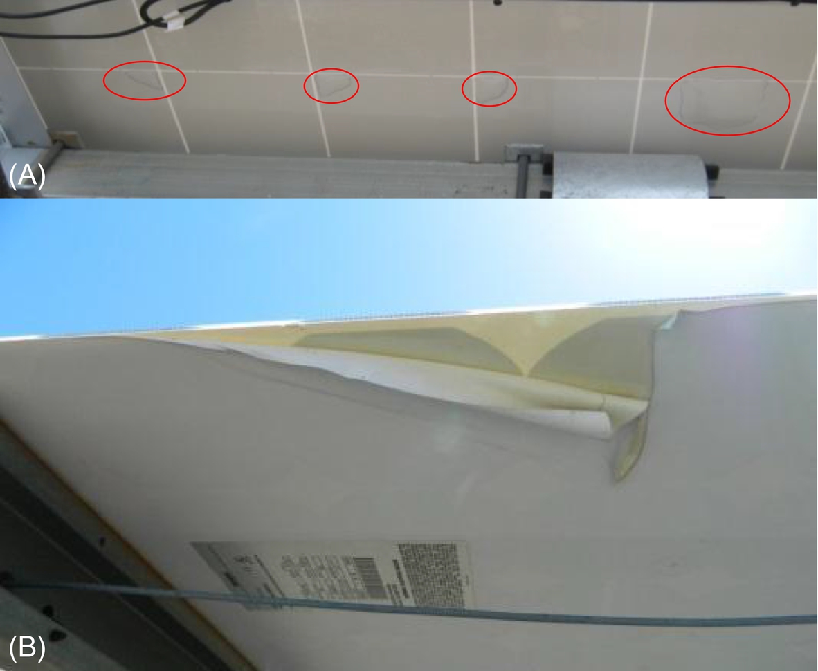
Similarly to discolouration, delamination at or near the front surface can be seen in a decreased Isc, at least in the initial stages, as an additional interface develops and loss of transmission occurs. If delamination continues and becomes more severe, moisture may ingress and lead to corrosion of the internal circuitry that can be observable in decreased fill factor (FF). Furthermore, delamination can also occur behind the x-Si cells and may manifest itself as bubbling of the backsheet or complete delamination (Fig. 3.12).
Metallization corrosion
Discolouration of the internal circuitry or corrosion is often preceded by delamination. Initially, the power loss is caused by the added interface. However, over time with increasing delamination, moisture can penetrate and lead to corrosion of the metallic circuitry. Visually corrosion is easily detectable, as shown in Fig. 3.11. Electrically, the power loss is typically associated with FF loss through increased series resistance (Fig. 3.13).

Potential-induced degradation
Module degradation as a function of the position in the string was first reported on high-efficiency n-type Si modules [47]. The initial confusing effect was that modules that were exposed to more positive bias displayed higher degradation. Although not fully understood at the time, the remedy was grounding and avoidance of positive bias. Only a few years later a similar effect was discovered for p-type x-Si modules placed in negative bias [48]. While more is being learned in this rapidly developing field, the cause of the effect appears to be the migration of sodium ions into the semiconductor junction [49]. This potential-induced degradation (PID) and the partial reversal of the degradation have been of significant interest in the last few years because of the rapidity and severity of the effect in some cases. Module manufacturers routinely label their products as ‘PID resistant’ or ‘PID free’, though it is not always clear what tests were performed that led to said label. Two standard test methods have been defined in IEC/TS 62804.
Cracked cells and snail trails
Another common cause of loss of Isc can be broken cells. Even though cracked cells have become more common as cells have been thinned in recent years, there are few papers written specifically about cracked cells. Publications more commonly describe ‘snail trails’ (observed when the encapsulant has a different colour near the crack than elsewhere, Fig. 3.14) and conclude that these decorate cracked cells that lead to substantial power loss [51]. However, instead of identifying the cracked cells as the problem that needs to be fixed, often the snail trails are identified as ‘the problem’. We have not seen a report that directly links the snail trails to performance loss, but note that the snail trails provide a simple way to identify cracked cells. Some PV customers wish to eliminate all cell cracks, but if a cell cracks in such a way that every fragment remains connected, there may not be power loss. In order to reduce the silicon usage, and, therefore, module cost, we need to better understand how to avoid cracks, how to test for them, and how to identify whether some cracks are acceptable [52]. Electroluminescence is a useful tool for identifying cracked cells [53] (Fig. 3.15).


Hot-spots
As individual cells are serial connected in a module substring, the current flowing through the cells is the same. If one cell is shaded, that cell is reverse-biased, dissipating power and therefore leading to heating effects. Bypass diodes are connected in parallel and in the opposite direction to the PV cells limiting the power dissipating effect (Fig. 3.16).
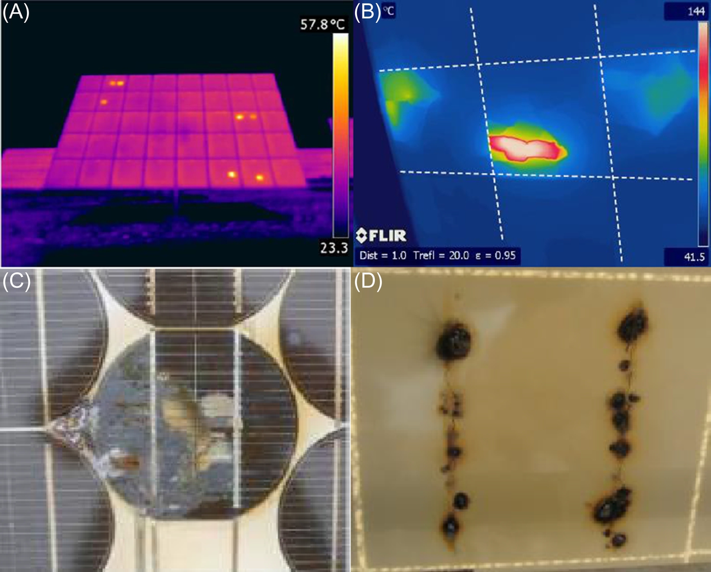
Partial shading is not the only situation that can lead to reverse bias of one or more cells. Mismatch between individual cells, eg, one cell producing less current than the other cells in a substring, can have a similar effect. The mismatch may increase during many years of field exposure as the individual cells degrade differently, exacerbating the effect. If the bypass diode fails to protect the substring, the heating can rapidly increase. Another ageing-related cause is the weakening connections of the internal module circuitry, such as solder bonds, through thermal cycling during field exposure. Finally, cracked cells may lead to hot-spots, as part of the cell is isolated and behaves similarly to a partially shaded cell. As the temperature difference between the hot-spot and the ambient area increases, safety becomes the primary concern. Significant damage to the front or the back of the module can occur, leading to elevated fire risk.
Glass
Glass breakage (Fig. 3.17) in thin-film modules is more common than in crystalline silicon because many thin-film products have annealed glass while most c-Si modules use tempered or heat-strengthened glass. Some arrays suffer from more glass breakage than others. Such glass breakage has been attributed to poor support structure design, inappropriate maintenance (eg, using a weed whacker to cut vegetation), poor installation and/or handling practices (eg, a small nick on the edge of a module can nucleate a crack) and finally manufacturing defects.

Frame
Bent frames are common (Fig. 3.18) in climates with snow and ice. The snow may partially melt and then refreeze along the bottom edge of the module, causing stress on the frame. Joerg Althaus has led an effort [56] to define IEC 62938 ‘Non-uniform snow load testing for PV modules’, planned for publication in 2016. This test will be valuable for those choosing modules for cold (icy) locations.

3.3.3 Standards development
Bankable PV (PV installations in which the investor has confidence in their reliable and long-term operation) benefits from international standards that address the module design, consistent manufacturing and system verification. The International PV Quality Assurance Task Force (PVQAT) was created to develop a set of universally accepted accelerated stress tests to identify adequate durability for all climates and mounting configurations [57]. PVQAT and IEC efforts to define improved PV standards are moving forward quickly to support the maturation of the industry. The challenge is to identify rapid test methods that adequately assess durability in a range of use environments while recognizing that quantitative lifetime assessment must be implemented for a specific bill of materials with a defined quality management system that specifies the variability allowed for the product implementation. PVQAT investigations will provide a basis for implementation of both climate-specific qualification tests and more quantitative service life predictions. Table 3.2 provides a summary of the module-level issues that were identified and the near- and long-term plans by PVQAT and Working Group 2 (WG2) (Modules) of IEC Technical Committee 82 (TC82) on PV.
Table 3.2
International standards efforts to address issues prioritized in Qualification Plus (Q+) [58]
| Priority | Current status | Near-term plan | Long-term plan |
| UV durability of polymeric components (encapsulants, backsheets, connectors and junction boxes) and as a requirement for insulation materials (see Q + component tests 1–4) | Recent and planned changes will add more UV and other testing of polymeric materials | (1) Submit 62788-7-2; (2) Submit amendment to IEC 61730 referencing IEC 62788-7-2 for materials weathering conditions; (3) Submit additional IEC 62788 parts; publish in 2016 | Define climate-specific UV exposures |
| Bypass diode and j-box thermal test (see Q + component test 5) | Multiple documents are in progress to address thermal endurance, cycling, and runaway | Five actions are described in text reference [55] | Define climate-specific diode tests |
| Electrical failures within the module (see Q + module test 1) | Ribbon interconnects can be tested with cyclic mechanical loading, but thermal cycling (TC) is still needed | Define climate-specific thermal-cycle tests and implementation within QMS | |
| Power loss from cracked cells (see Q + module test 2) | IEC 62782 TS: Cyclic (dynamic) mechanical load testing and IEC 62759-1 PV modules— Transportation testing were published | Submit amendment to IEC 61215 to add 1000 cycles from IEC 62782 before TC and humidity freeze | Define climate-specific tests for cracked cells, if needed |
| Susceptibility to PID (see Q + module test 3) | IEC/TS 62804-1 Test methods for detection of PID—Part 1 Crystalline Silicon has been published | Define standard labels for PID susceptibility | Understand relationship between degradation in the test and in the field; Identify quick tests for screening cells and encapsulant materials |
| Susceptibility to hot spot degradation (see Q + module test 4) | Revised hot-spot test is included in 2016 version of IEC 61215 | Define improved hot-spot test for thin-film modules | |
| Improve confidence in Quality Management System (QMS) (see Q + description of sampling and QMS) | IEC/TS 62941 Guideline for increased confidence in PV module design qualification and type approval was published | Implement through IECRE | Facilitate adoption and assess value of extending to quantitative assessment |
| Structural failure from snow and ice (based on experience in Europe and New England) | IEC 62938 Non-uniform snow load testing for PV modules Committee Draft has been reviewed | Complete IEC 62938; publish in 2017 | Encourage use of the snow load test to differentiate modules |
| Faster degradation in hot climates | Delamination, encapsulant discolouration, and thermal fatigue are documented to increase with high temperature | Define difference in use environment | Use IEC 62892 to implement comprehensive tests at higher temperatures |
| Assessment of system functionality | Drafts completed for both energy and capacity tests | Publication of IEC 61724-2 and IEC 61724-3 in 2016 | Implement as part of IECRE |

3.4 Conclusion and future trends
Today, the PV industry is fairly knowledgeable about the most common causes of failures in the field, but a complete understanding of the acceptable process and design windows is challenging, especially as companies may make changes to the bill of materials frequently. PV reliability standards are maturing by:
• addressing failure mechanisms that have recently become problematic;
• differentiating the durability of PV module designs as a function of the use environment and
• improving manufacturing consistency toward a consistent implementation of product design, moving toward inclusion of service life prediction in the most mature quality management systems.
Today's most critical issues will be addressed by standards completed in 2016. Quantitative service life predictions will become practical when the industry is mature enough for product designs to stabilize enough to allow time for testing and model development and validation.
3.5 Resources
3.5.1 Visual inspection sheet