The extension to Logistic Regression, for classifying more than two classes, is Multiclass Logistic Regression. Its foundation is actually a generic approach: it doesn't just work for Logistic Regressors, it also works with other binary classifiers. The base algorithm is named One-vs-rest, or One-vs-all, and it's simple to grasp and apply.

Let's describe it with an example: we have to classify three kinds of flowers and, given some features, the possible outputs are three classes: f1, f2, and f3. That's not what we've seen so far; in fact, this is not a binary classification problem. Instead, it seems very easy to break down this problem into three simpler problems:

For all three problems, we can use a binary classifier, as Logistic Regressor, and, unsurprisingly, the first classifier will output P(y = f1|x); the second and the third will output respectively P(y = f2|x) and P(y = f3|x).

To make the final prediction, we just need to select the classifier that emitted the highest probability. Having trained three classifiers, the feature space is not divided in two subplanes, but according to the decision boundary of the three classifiers.

The approach of One-vs-all is very convenient, in fact:

For a better understanding, let's make a multiclass classification example, creating a dummy three-class dataset, splitting it as training and test sets, training a Multiclass Logistic Regressor, applying it on the training set, and finally visualizing the boundaries:

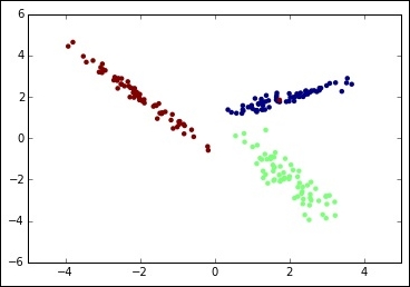
In:
%reset -f
In:
%matplotlib inline

import matplotlib.pyplot as plt
from sklearn.datasets import make_classification

X, y = make_classification(n_samples=200, n_features=2,
                           n_classes=3, n_informative=2,
                           n_redundant=0, n_clusters_per_class=1,
                           class_sep = 2.0, random_state=101)

plt.scatter(X[:, 0], X[:, 1], marker='o', c=y, linewidth=0, edgecolor=None)
plt.show()
Out:

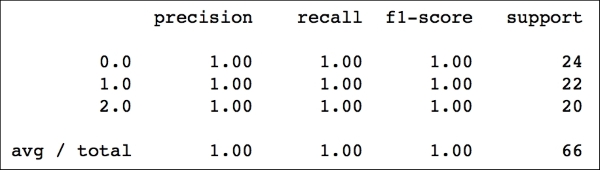
In:
from sklearn.cross_validation import train_test_split

X_train, X_test, y_train, y_test = train_test_split(X, y.astype(float),
                                   test_size=0.33, random_state=101)
In:
from sklearn.linear_model import LogisticRegression

clf = LogisticRegression()
clf.fit(X_train, y_train.astype(int))
y_clf = clf.predict(X_test)
In:
from sklearn.metrics import classification_report
print(classification_report(y_test, y_clf))
Out:

In:
import numpy as np

h = .02  # step size in the mesh

x_min, x_max = X[:, 0].min() - .5, X[:, 0].max() + .5
y_min, y_max = X[:, 1].min() - .5, X[:, 1].max() + .5
xx, yy = np.meshgrid(np.arange(x_min, x_max, h), np.arange(y_min, y_max, h))
Z = clf.predict(np.c_[xx.ravel(), yy.ravel()])

# Put the result into a color plot
Z = Z.reshape(xx.shape)
plt.pcolormesh(xx, yy, Z, cmap=plt.cm.autumn)

# Plot also the training points
plt.scatter(X[:, 0], X[:, 1], c=y, edgecolors='k', cmap=plt.cm.Paired)
plt.xlim(xx.min(), xx.max())
plt.ylim(yy.min(), yy.max())
plt.xticks(())
plt.yticks(())

plt.show()
Out:

On this dummy dataset, the classifier has achieved a perfect classification (precision, recall, and f1-score are all 1.0). In the last picture, you can see that the decision boundaries define three areas, and create a non-linear division.

Finally, let's observe the first feature vector, its original label, and its predicted label (both reporting class "0"):

In:
print(X_test[0])
print(y_test[0])
print(y_clf[0])
Out:
[ 0.73255032  1.19639333]
0.0
0

To get its probabilities to belong to each of the three classes, you can simply apply the predict_proba method (exactly as in the binary case), and the classifier will output the three probabilities. Of course, their sum is 1.0, and the highest value is, naturally, one for class "0".

In:
clf.predict_proba(X_test[0])
Out:
array([[ 0.72797056,  0.06275109,  0.20927835]])