Let's gradually introduce how logistic regression works. We said that it's a classifier, but its name recalls a regressor. The element we need to join the pieces is the probabilistic interpretation.

In a binary classification problem, the output can be either "0" or "1". What if we check the probability of the label belonging to class "1"? More specifically, a classification problem can be seen as: given the feature vector, find the class (either 0 or 1) that maximizes the conditional probability:

Here's the connection: if we compute a probability, the classification problem looks like a regression problem. Moreover, in a binary classification problem, we just need to compute the probability of membership of class "1", and therefore it looks like a well-defined regression problem. In the regression problem, classes are no longer "1" or "0" (as strings), but 1.0 and 0.0 (as the probability of belonging to class "1").

Let's now try fitting a multiple linear regressor on a dummy classification problem, using a probabilistic interpretation. We reuse the same dataset we created earlier in this chapter, but first we split the dataset into train and test sets, and we convert the y vector to floating point values:

In:
from sklearn.cross_validation import train_test_split

X_train, X_test, y_train, y_test = train_test_split(X, y.astype(float),	est_size=0.33, random_state=101)

In:
y_test.dtype
Out:
dtype('float64')
In:
y_test
Out:

Here, with these few methods, we split the datasets into two folds, (train and test) and we converted all the numbers in the y array to floating point. In the last cell, we effectively check the operation. Now, if y = 1.0, it means that the relative observation is 100% class "1"; y = 0.0 implies that the observation is 0% class "1". Since it's a binary classification task, it implies that it's also 100% class "0" (note that the percentages here refer to probability).

Let's now proceed with the regression:

In:
from sklearn.linear_model import LinearRegression
regr = LinearRegression()
regr.fit(X_train, y_train)
regr.predict(X_test)
Out:

The output—that is, the prediction of the regressor—should be the probability of belonging to class 1. As you can see in the last cell output, that's not a proper probability, since it contains values below 0 and greater than 1. The simplest idea here is clipping results between 0 and 1, and putting a threshold at 0.5: if the value is >0.5, then the predicted class is "1"; otherwise the predicted class is "0".

This procedure works, but we can do better. We've seen how easy it is to transit from a classification problem to a regression one, and then go back with predicted values to predicted classes. With this process in mind, let's again start the analysis, digging further in its core algorithm while introducing some changes.

In our dummy problem, we applied the linear regression model to estimate the probability of the observation belonging to class "1". The regression model was (as we've seen in the previous chapter):

Now, we've seen that the output is not a proper probability. To be a probability, we need to do the following:

To have both conditions true, the best we could do is to send the output of the regressor through a sigmoid curve, or an S-shaped curve. A sigmoid generically maps values in R (the field of real numbers) to values in the range [0,1], and its value when mapping 0 is 0.5.

On the basis of such a hypothesis, we can now write (for the first time) the formula underneath the logistic regression algorithm.

Note also that the weight W[0] (the bias weight) will take care of the misalignment of the central point of the sigmoid (it's in 0, whereas the threshold is in 0.5).

That's all. That's the logistic regression algorithm. There is just one thing missing: why logistic? What's the σ function?

Well, the answer to both questions is trivial: the standard choice of sigma is the logistic function, also named the inverse-logit function:

Although there are infinite functions that satisfy the sigmoid constraints, the logistic has been chosen because it's continuous, easily differentiable, and quick to compute. If the results are not satisfactory, always consider that, by introducing a couple of parameters, you can change the steepness and the center of the function.

The sigmoid function is quickly drawn:

In:
import numpy as np

def model(x):
    return 1 / (1 + np.exp(-x))

X_vals = np.linspace(-10, 10, 1000)
plt.plot(X_vals, model(X_vals), color='blue', linewidth=3)
plt.ylabel('sigma(t)')
plt.xlabel('t')

plt.show()
Out:

You can immediately see that, for a very low t, the function tends to the value 0; for a very high t, the function tends to be 1, and, in the center, where t is 0, the function is 0.5. Exactly the sigmoid function we were looking for.

More on the logistic and logit functions

Now, why did we use the inverse of the logit function? Isn't there anything better than that? The answer to this question comes from statistics: we're dealing with probabilities, and the logit function is a great fit. In statistics, the logit function applied to a probability, returns the log-odds:

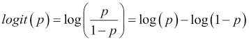
This function transforms numbers from range [0,1] to numbers in (−∞, +∞).

Now, let's see if you can intuitively understand the logic behind the selection of the inverse-logit function as the sigmoid function for the logistic regression. Let's first write down the probabilities for both classes, according to this logistic regression equation:

Let's now compute the log-odds:

However, not surprisingly, that's also the logit function, applied to the probability of getting a "1":

The chain of our reasoning is finally closed, and here's why logistic regression is based on, as the definition implies, the logistic function. Actually, logistic regression is a model of the big category of the GLM: the generalized linear model. Each model has a different function, a different formulation, a different operative hypothesis, and not, surprisingly, a different goal.

Let's see some code

First, we start with the dummy dataset we created at the beginning of the chapter. Creating and fitting a logistic regressor classifier is really easy: thanks to Scikit-learn, it just requires a couple of lines of Python code. As for regressors, to train the model you need to call the fit method, whereas for predicting the class you just need to call the predict method:

In:
from sklearn.linear_model import LogisticRegression

clf = LogisticRegression()
clf.fit(X_train, y_train.astype(int))
y_clf = clf.predict(X_test)

print(classification_report(y_test, y_clf))
Out:

Note that here we're not making a regression operation; that's why the label vector must comprise integers (or class indexes). The report shown at the bottom shows a very accurate prediction: all the scores are close to 1 for all classes. Since we have 33 samples in the test set, 0.97 means just one case misclassified. That's almost perfect in this dummy example!

Now, let's try to dig under the hood even more. First, we would like to check the decision boundary of the classifier: which part of the bidimensional space has points being classified as "1"; and where are the "0"s? Let's see how you can visually see the decision boundary here:

In:
# Example based on:
# Code source: Gaël Varoquaux, Modified for documentation by Jaques Grobler, License: BSD 3 clause

h = .02  # step size in the mesh

# Plot the decision boundary. For that, we will assign a color to each
# point in the mesh [x_min, m_max]x[y_min, y_max].
x_min, x_max = X[:, 0].min() - .5, X[:, 0].max() + .5
y_min, y_max = X[:, 1].min() - .5, X[:, 1].max() + .5
xx, yy = np.meshgrid(np.arange(x_min, x_max, h), np.arange(y_min, y_max, h))
Z = clf.predict(np.c_[xx.ravel(), yy.ravel()])

# Put the result into a color plot
Z = Z.reshape(xx.shape)
plt.pcolormesh(xx, yy, Z, cmap=plt.cm.autumn)

# Plot also the training points
plt.scatter(X[:, 0], X[:, 1], c=y, edgecolors='k', linewidth=0, cmap=plt.cm.Paired)

plt.xlim(xx.min(), xx.max())
plt.ylim(yy.min(), yy.max())
plt.xticks(())
plt.yticks(())

plt.show()
Out:

The separation is almost vertical. "1"s are on the left (yellow) side; "0"s on the right (red). From the earlier screenshot, you can immediately perceive the misclassification: it's pretty close to the boundary. Therefore, its probability of belonging to class "1" will be very close to 0.5.

Let's now see the bare probabilities and the weight vector. To compute the probability, you need to use the predict_proba method of the classifier. It returns two values for each observation: the first is the probability of being of class "0"; the second the probability for class "1". Since we're interested in class "1", here we just select the second value for all the observations:

In:
Z = clf.predict_proba(np.c_[xx.ravel(), yy.ravel()])[:,1]
Z = Z.reshape(xx.shape)
plt.pcolormesh(xx, yy, Z, cmap=plt.cm.autumn)

ax = plt.axes()
ax.arrow(0, 0, clf.coef_[0][0], clf.coef_[0][1], head_width=0.5, 
head_length=0.5, fc='k', ec='k')
plt.scatter(0, 0, marker='o', c='k')

plt.xlim(xx.min(), xx.max())
plt.ylim(yy.min(), yy.max())

plt.show()
Out:

In the screenshot, pure yellow and pure red are where the predicted probability is very close to 1 and 0 respectively. The black dot is the origin (0,0) of the Cartesian bidimensional space, and the arrow is the representation of the weight vector of the classifier. As you can see, it's orthogonal to the decision boundary, and it's pointing toward the "1" class. The weight vector is actually the model itself: if you need to store it in a file, consider that it's just a couple of floating point numbers and nothing more.

Lastly, I'd want to focus on speed. Let's now see how much time the classifier takes to train and to predict the labels:

In:
%timeit clf.fit(X, y)
Out:
1000 loops, best of 3: 291 µs per loop
In:
%timeit clf.predict(X)
Out:
10000 loops, best of 3: 45.5 µs per loop
In:
%timeit clf.predict_proba(X)
Out:
10000 loops, best of 3: 74.4 µs per loop

Although timings are computer-specific (here we're training it and predicting using the full 100-point dataset), you can see that Logistic Regression is a very fast technique both during training and when predicting the class and the probability for all classes.