
Having set up all your working tools (directly installing Python and IPython or using a scientific distribution), you are now ready to start using linear models to incorporate new abilities into the software you plan to build, especially predictive capabilities. Up to now, you have developed software solutions based on certain specifications you defined (or specifications that others have handed to you). Your approach has always been to tailor the response of the program to particular inputs, by writing code carefully mapping every single situation to a specific, predetermined response. Reflecting on it, by doing so you were just incorporating practices that you (or others) have learned from experience.
However, the world is complex, and sometimes your experience is not enough to make your software smart enough to make a difference in a fairly competitive business or in challenging problems with many different and mutable facets.
In this chapter, we will start exploring an approach that is different from manual programming. We are going to present an approach that enables the software to self-learn the correct answers to particular inputs, provided you can define the problem in terms of data and target response and that you can incorporate in the processes some of your domain expertise—for instance, choosing the right features for prediction. Therefore, your experience will go on being critical when it comes to creating your software, though in the form of learning from data. In fact, your software will be learning from data accordingly to your specifications. We are also going to illustrate how it is possible to achieve this by resorting to one of the simplest methods for deriving knowledge from data: linear models.
Specifically, in this chapter, we are going to discuss the following topics:
- Understanding what problems machine learning can solve
- What problems a regression model can solve
- The strengths and weaknesses of correlation
- How correlations extends to a simple regression model
- The when, what, and why of a regression model
- The essential mathematics behind gradient descent
In the process, we will be using some statistical terminology and concepts in order to provide you with the prospect of linear regression in the larger frame of statistics, though our approach will remain practical, offering you the tools and hints to start building linear models using Python and thus enrich your software development.
Thanks to machine learning algorithms, deriving knowledge from data is possible. Machine learning has solid roots in years of research: it has really been a long journey since the end of the fifties, when Arthur Samuel clarified machine learning as being a "field of study that gives computers the ability to learn without being explicitly programmed."
The data explosion (the availability of previously unrecorded amounts of data) has enabled the widespread usage of both recent and classic machine learning techniques and made them high-performance techniques. If nowadays you can talk by voice to your mobile phone and expect it to answer properly to you, acting as your secretary (such as Siri or Google Now), it is uniquely because of machine learning. The same holds true for every application based on machine learning such as face recognition, search engines, spam filters, recommender systems for books/music/movies, handwriting recognition, and automatic language translation.
Some other actual usages of machine learning algorithms are somewhat less obvious, but nevertheless important and profitable, such as credit rating and fraud detection, algorithmic trading, advertising profiling on the Web, and health diagnostics.
Generally speaking, machine learning algorithms can learn in three ways:
- Supervised learning: This is when we present labeled examples to learn from. For instance, when we want to be able to predict the selling price of a house in advance in a real estate market, we can get the historical prices of houses and have a supervised learning algorithm successfully figure out how to associate the prices to the house characteristics.
- Unsupervised learning: This is when we present examples without any hint, leaving it to the algorithm to create a label. For instance, when we need to figure out how the groups inside a customer database can be partitioned into similar segments based on their characteristics and behaviors.
- Reinforcement learning: This is when we present examples without labels, as in unsupervised learning, but get feedback from the environment as to whether label guessing is correct or not. For instance, when we need software to act successfully in a competitive setting, such as a videogame or the stock market, we can use reinforcement learning. In this case, the software will then start acting in the setting and it will learn directly from its errors until it finds a set of rules that ensure its success.
Unsupervised learning has important applications in robotic vision and automatic feature creation, and reinforcement learning is critical for developing autonomous AI (for instance, in robotics, but also in creating intelligent software agents); however, supervised learning is most important in data science because it allows us to accomplish something the human race has aspired to for ages: prediction.
Prediction has applications in business and for general usefulness, enabling us to take the best course of action since we know from predictions the likely outcome of a situation. Prediction can make us successful in our decisions and actions, and since ancient times has been associated with magic or great wisdom.
Supervised learning is no magic at all, though it may look like sorcery to some people, as Sir Arthur Charles Clarke stated, "any sufficiently advanced technology is indistinguishable from magic." Supervised learning, based on human achievements in mathematics and statistics, helps to leverage human experience and observations and turn them into precise predictions in a way that no human mind could. However, supervised learning can predict only in certain favorable conditions. It is paramount to have examples from the past at hand from which we can extract rules and hints that can support wrapping up a highly likely prediction given certain premises.
In one way or another, no matter the exact formulation of the machine learning algorithm, the idea is that you can tell the outcome because there have been certain premises in the observed past that led to particular conclusions.
In mathematical formalism, we call the outcome we want to predict the response or target variable and we usually label it using the lower case letter y.
The premises are instead called the predictive variables, or simply attributes or features, and they are labeled as a lowercase x if there is a single one and by an uppercase X if there are many. Using the uppercase letter X we intend to use matrix notation, since we can also treat the y as a response vector (technically a column vector) and the X as a matrix containing all values of the feature vectors, each arranged into a separate column of the matrix.
It is also important to always keep a note of the dimensions of X and y; thus, by convention, we can call n the number of observations and p the number of variables. Consequently our X will be a matrix of size (n, p), and our y will always be a vector of size n.
We can affirm that, when we are learning to predict from data in a supervised way, we are actually building a function that can answer the question about how X can imply y.
Using these new matrix symbolic notations, we can define a function, a functional mapping that can translate X values into y without error or with an acceptable margin of error. We can affirm that all our work will be to determinate a function of the following kind:
When the function is specified, and we have in mind a certain algorithm with certain parameters and an X matrix made up of certain data, conventionally we can refer to it as a hypothesis. The term is suitable because we can intend our function as a ready hypothesis, set with all its parameters, to be tested if working more or less well in predicting our target y.
Before talking about the function (the supervised algorithm that does all the magic), we should first spend some time reasoning about what feeds the algorithm itself. We have already introduced the matrix X, the predictive variables, and the vector y, the target answer variable; now it is time to explain how we can extract them from our data and what exactly their role is in a learning algorithm.
Reflecting on the role of your predictive variable in a supervised algorithm, there are a few caveats that you have to keep in mind throughout our illustrations in the book, and yes, they are very important and decisive.
To store the predictive variables, we use a matrix, usually called the X matrix:

In this example, our X is made up of only one variable and it contains n cases (or observations).
Tip
If you would like to know when to use a variable or feature, just consider that in machine learning feature and attribute are terms that are favored over variable, which has a definitively statistical flavor hinting at something that varies. Depending on the context and audience, you can effectively use one or the other.
In Python code, you can build a one-column matrix structure by typing:
In: import numpy as np
  vector = np.array([1,2,3,4,5])
  row_vector = vector.reshape((5,1))
  column_vector = vector.reshape((1,5))
  single_feature_matrix = vector.reshape((1,5))
Using the NumPy array we can quickly derive a vector and a matrix. If you start from a Python list, you will get a vector (which is neither a row nor a column vector, actually). By using the reshape method, you can transform it into a row or column vector, based on your specifications.
Real-world data usually need matrices that are more complex, and real-world matrices comprise uncountable different data columns (the variety element of big data). Most likely, a standard X matrix will have more columns, so the notation we will be referring to is:
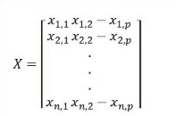
Now, our matrix has more variables, all p variables, so its size is n x p. In Python, there are two methods to make up such a data matrix:
In: multiple_feature_matrix =
np.array([[1,2,3,4,5],[6,7,8,9,10],[11,12,13,14,15]])
You just have to transform with the array function a list of lists, where each internal list is a row matrix; or you create a vector with your data and then reshape it in the shape of your desired matrix:
In: multiple_feature_matrix = np.array([[1,2,3,4,5],[6,7,8,9,10],[11,12,13,14,15]])
The information present in the set of observations from the past, that we are using as X, can deeply affect how we are going to build the link between our X and the y.
In fact, usually it is the case that we do not know the full range of possible associations between X and y because:
- We have just observed a certain X, so our experience of y for a given X is biased, and this is a sampling bias because, as in a lottery, we have drawn only certain numbers in a game and not all the available ones
- We never observed certain (X, y) associations (please note the formulation in a tuple, indicating the interconnection between X and y), because they never happened before, but that does not exclude them from happening in the future (and incidentally we are striving to forecast the future)
There is little to do with the second problem, (we can extrapolate the future only through the directions pointed out by the past), but you can actually check how recent the data you are using is. If you are trying to forecast in a context that is very susceptible to changes and mutable from day to day, you have to keep in mind that your data could quickly become outdated and you may be unable to guess new trends. An example of a mutable context where we constantly need to update models is the advertising sector (where the competitive scenery is frail and continually changing). Consequently, you continually need to gather fresher data that could allow you to build a much more effective supervised algorithm.
As for the first problem, you can solve it using more and more cases from different sources. The more you sample, the more likely your drawn set of X will resemble a complete set of possible and true associations of X with y. This is understandable via an important idea in probability and statistics: the law of large numbers.
The law of large numbers suggests that, as the number of your experiments grows, so the likelihood that the average of their results will represent the true value (that the experiments themselves are trying to figure out) will increase.
Supervised algorithms learn from large samples of historical data, called batches, fetched all at once from large data repositories, such as databases or data lakes. Alternatively, they also could pick the examples that are most useful for their learning by themselves and ignore the bulk of the data (this is called active learning and it is a kind of semi-supervised learning that we won't discuss here).
If our environment is fast-paced, they also could just stream data as it is available, continuously adapting to any new association between the predictive variables and the response (this is called online learning and we will discuss it in Chapter 7, Online and Batch Learning).
Another important aspect of the X matrix of predictors to be considered is that up to now we assumed that we could deterministically derive the response y using the information in the matrix X. Unfortunately this is not always so in the real world and it is not rare that you actually try to figure out your response y using a completely wrong set of predictive X. In such cases, you have to figure out that you are actually wasting your time in trying to fit something working between your X and y and that you should look for some different X (again more data in the sense of more variables).
According to the model used, having more variables and cases is usually beneficial under different points of view. More cases reduces the possibility of learning from a biased and limited set of observations. Many algorithms can better estimate their internal parameters (and produce more accurate predictions) if trained using large sets of observations. Also, having more variables at hand can be beneficial, but in the sense that it increases the chance of having explicative features to be used for machine learning. Many algorithms are in fact sensitive to redundant information and noise present in features, consequently requiring some feature selection to reduce the predictors involved in the model. This is quite the case with linear regression, which can surely take advantage of more cases for its training, but it should also receive a parsimonious and efficient set of features to perform at its best. Another important aspect to know about the X matrix is that it should be made up solely of numbers. Therefore, it really matters what you are working with. You can work with the following:
- Physical measurements, which are always OK because they are naturally numbers (for example, height)
- Human measurements, which are a bit less OK, but are still fine when they have a certain order (that is, all numbers that we give as scores based on our judgment) and so they can be converted into rank numbers (such as 1, 2, and 3 for the first, second, and third values, and so on)
We call such values quantitative measurements. We expect quantitative measurement to be continuous and that means a quantitative variable can take any real positive or negative number as a valid value. Human measurements are usually only positive, starting from zero or one, so it is just a fair approximation to consider them quantitative.
For physical measurements, in statistics, we distinguish between interval and ratio variables. The difference is that ratio variables have a natural zero whereas in interval data the zero is an arbitrary one. A good example is temperature; in fact, unless you use the Kelvin scale, whose zero is an absolute one, both Fahrenheit and Celsius have arbitrary scales. The main implication is about the ratios (if the zero is arbitrary, the ratio is also arbitrary).
Human measurements that are numerical are called ordinal variables. Unlike interval data, ordinal data does not have a natural zero. Moreover, the interval between each value on an interval scale is equal and regular; however, in an ordinal scale, though the distance between the values is the same, their real distance could be very different. Let's think of a scale made of three textual values: good, average, and bad. Next, let's say that we arbitrarily decide that good is 3, average is 2, and bad is 1. We call this arbitrary assignment of values ordinal encoding. Now, from a mathematical point of view, though the interval between 3 and 2 in respect of the interval from 2 to 1 is the same (that is, one point), are we really sure that the real distance between good and average is the same as that from average and bad? For instance, in terms of customer satisfaction, does it costs the same effort going from an evaluation of bad to one of average and from one of average to one of excellent?
Qualitative measurements (for example, a value judgment such as good, average, or bad, or an attribute such as being colored red, green, or blue) need some work to be done, some clever data manipulation, but they can still be part of our X matrix using the right transformation. Even more unstructured qualitative information (such as text, sound, or a drawing) can be transformed and reduced to a pool of numbers and can be ingested into an X matrix.
Qualitative variables can be stored as numbers into single-value vectors or they can have a vector for each class. In such a case, we are talking about binary variables (also called dummy variables in statistical language).
We are going to discuss in greater detail how to transform the data at hand, especially if its type is qualitative, into an input matrix suitable for supervised learning in Chapter 5, Data Preparation.
As a starting point before working on the data itself, it is necessary to question the following:
- The quality of the data—that is, whether the data available can really represent the right information pool for extracting X-y rules
- The quantity of data—that is, checking how much data is available, keeping in mind that, for building robust machine learning solutions, it is safer to have a large variety of variables and cases (at least when you're dealing with thousands of examples)
- The extension of data in time—that is, checking how much time the data spans in the past (since we are learning from the past)
Reflecting on the role of the response variable, our attention should be first drawn to what type of variable we are going to predict, because that will distinguish the type of supervised problem to be solved.
If our response variable is a quantitative one, a numeric value, our problem will be a regression one. Ordinal variables can be solved as a regression problem, especially if they take many different distinct values. The output of a regression supervised algorithm is a value that can be directly used and compared with other predicted values and with the real response values used for learning.
For instance, as an example of a regression problem, in the real estate business a regression model could predict the value of a house just from some information about its location and its characteristics, allowing an immediate discovery of market prices that are too cheap or too expensive by using the model's predictions as an indicator of a fair fact-based estimation (if we can reconstruct the price by a model, it is surely well justified by the value of the measurable characteristics we used as our predictors).
If our response variable is a qualitative one, our problem is one of classification. If we have to guess between just two classes, our problem is called a binary classification; otherwise, if more classes are involved, it is a called a multi-label classification problem.
For instance, if we want to guess the winner in a game between two football teams, we have a binary classification problem because we just need to know if the first team will win or not (the two classes are team wins, team loses). A multi-label classification could instead be used to predict which football team among a certain number will win (so in our prediction, the classes to be guessed are the teams).
Ordinal variables, if they do not take many distinct values, can be solved as a multi-label classification problem. For instance, if you have to guess the final ranking of a team in a football championship, you could try to predict its final position in the leader board as a class. Consequently, in this ordinal problem you have to guess many classes corresponding to different positions in the championship: class 1 could represent the first position, class 2 the second position, and so on. In conclusion, you could figure the final ranking of a team as the positional class whose likelihood of winning is the greatest.
As for the output, classification algorithms can provide both classification into a precise class and an estimate of the probability of being part of any of the classes at hand.
Continuing with examples from the real estate business, a classification model could predict if a house could be a bargain or if it could increase its value given its location and its characteristics, thus allowing a careful investment selection.
The most noticeable problem with response variables is their exactness. Measurement errors in regression problems and misclassification in classification ones can damage the ability of your model to perform well on real data by providing inaccurate information to be learned. In addition, biased information (such as when you provide cases of a certain class and not from all those available) can hurt the capacity of your model to predict in real-life situations because it will lead the model to look at data from a non-realistic point of view. Inaccuracies in the response variable are more difficult and more dangerous for your model than problems with your features.
For single predictors, the outcome variable y is also a vector. In NumPy, you just set it up as a generic vector or as a column vector:
In: y = np.array([1,2,3,4,5]).reshape((5,1))
The family of linear models is so named because the function that specifies the relationship between the X, the predictors, and the y, the target, is a linear combination of the X values. A linear combination is just a sum where each addendum value is modified by a weight. Therefore, a linear model is simply a smarter form of a summation.
Of course there is a trick in this summation that makes the predictors perform like they do while predicting the answer value. As we mentioned before, the predictors should tell us something, they should give us some hint about the answer variable; otherwise any machine learning algorithm won't work properly. We can predict our response because the information about the answer is already somewhere inside the features, maybe scattered, twisted, or transformed, but it is just there. Machine learning just gathers and reconstructs such information.
In linear models, such inner information is rendered obvious and extracted by the weights used for the summation. If you actually manage to have some meaningful predictors, the weights will just do all the heavy work to extract it and transform it into a proper and exact answer.
Since the X matrix is a numeric one, the sum of its elements will result in a number itself. Linear models are consequently the right tool for solving any regression problem, but they are not limited to just guessing real numbers. By a transformation of the response variable, they can be enabled to predict counts (positive integer numbers) and probabilities relative to being part of a certain group or class (or not).
In statistics, the linear model family is called the generalized linear model (GLM). By means of special link functions, proper transformation of the answer variable, proper constraints on the weights and different optimization procedures (the learning procedures), GLM can solve a very wide range of different problems. In this book, our treatise won't extend beyond what is necessary to the statistical field. However, we will propose a couple of models of the larger family of the GLM, namely linear regression and logistic regression; both methods are appropriate to solve the two most basic problems in data science: regression and classification.
Because linear regression does not require any particular transformation of the answer variable and because it is conceptually the real foundation of linear models, we will start by understanding how it works. To make things easier, we will start from the case of a linear model using just a single predictor variable, a so-called simple linear regression. The predictive power of a simple linear regression is very limited in comparison with its multiple form, where many predictors at once contribute to the model. However, it is much easier to understand and figure out its functioning.
We provide some practical examples in Python throughout the book and do not leave explanations about the various regression models at a purely theoretical level. Instead, we will explore together some example datasets, and systematically illustrate to you the commands necessary to achieve a working regression model, interpret its structure, and deploy a predicting application.
For the initial presentation of the linear regression in its simple version (using only one predictive variable to forecast the response variable), we have chosen a couple of datasets relative to real estate evaluation.
Real estate is quite an interesting topic for an automatic predictive model since there is quite a lot of freely available data from censuses and, being an open market, even more data can be scraped from websites monitoring the market and its offers. Moreover, because the renting or buying of a house is quite an important economic decision for many individuals, online services that help to gather and digest the large amounts of available information are indeed a good business model idea.
The first dataset is quite a historical one. Taken from the paper by Harrison, D. and Rubinfeld, D.L. Hedonic Housing Prices and the Demand for Clean Air (J. Environ. Economics & Management, vol.5, 81-102, 1978), the dataset can be found in many analysis packages and is present at the UCI Machine Learning Repository (https://archive.ics.uci.edu/ml/datasets/Housing).
The dataset is made up of 506 census tracts of Boston from the 1970 census and it features 21 variables regarding various aspects that could impact real estate value. The target variable is the median monetary value of the houses, expressed in thousands of USD. Among the available features, there are some fairly obvious ones such as the number of rooms, the age of the buildings, and the crime levels in the neighborhood, and some others that are a bit less obvious, such as the pollution concentration, the availability of nearby schools, the access to highways, and the distance from employment centers.
The second dataset from the Carnegie Mellon University Statlib repository (https://archive.ics.uci.edu/ml/datasets/Housing) contains 20,640 observations derived from the 1990 US Census. Each observation is a series of statistics (9 predictive variables) regarding a block group—that is, approximately 1,425 individuals living in a geographically compact area. The target variable is an indicator of the house value of that block (technically it is the natural logarithm of the median house value at the time of the census). The predictor variables are basically median income.
The dataset has been used in Pace and Barry (1997), Sparse Spatial Autoregressions, Statistics and Probability Letters, (http://www.spatial-statistics.com/pace_manuscripts/spletters_ms_dir/statistics_prob_lets/pdf/fin_stat_letters.pdf), a paper on regression analysis including spatial variables (information about places including their position or their nearness to other places in the analysis). The idea behind the dataset is that variations of house values can be explained by exogenous variables (that is, external to the house itself) representing population, the density of buildings, and the population's affluence aggregated by area.
The code for downloading the data is as follows:
In: from sklearn.datasets import fetch_california_housing
  from sklearn.datasets import load_boston
  boston = load_boston()
  california = fetch_california_housing()
We will be exclusively using the Boston dataset in this and the following chapters, but you can explore the California one and try to replicate the analysis done on the Boston one. Please remember to use the preceding code snippet before running any other code or you won't have the boston and california variables available for analysis.