
Numeric features can be transformed, regardless of the target variable. This is often a prerequisite for better performance of certain classifiers, particularly distance-based. We usually avoid ( besides specific cases such as when modeling a percentage or distributions with long queues) transforming the target, since we will make any pre-existent linear relationship between the target and other features non-linear.
We will keep on working on the Boston Housing dataset:
In: import numpy as np
  boston = load_boston()
  labels = boston.feature_names
  X = boston.data
  y = boston.target
  print (boston.feature_names)

Out: ['CRIM' 'ZN' 'INDUS' 'CHAS' 'NOX' 'RM' 'AGE' 'DIS' 'RAD' 'TAX' 'PTRATIO' 'B' 'LSTAT']
As before, we fit the model using LinearRegression from Scikit-learn, this time measuring its R-squared value using the r2_score function from the metrics module:
In: linear_regression = linear_model.LinearRegression(fit_intercept=True)
  linear_regression.fit(X, y)

  from sklearn.metrics import r2_score
  print ("R-squared: %0.3f" % r2_score(y, linear_regression.predict(X)))

Out: R-squared: 0.741
Residuals are what's left from the original response when the predicted value is removed. It is numeric information telling us what the linear model wasn't able to grasp and predict by its set of coefficients and intercepts.
Obtaining residuals when working with Scikit-learn requires just one operation:
In: residuals = y - linear_regression.predict(X)
  print ("Head of residual %s" % residuals[:5])
  print ("Mean of residuals: %0.3f" % np.mean(residuals))
  print ("Standard deviation of residuals: %0.3f" \% np.std(residuals))

Out: Head of residual [-6.00821 -3.42986  4.12977  4.79186  8.25712]
    Mean of residuals: 0.000
    Standard deviation of residuals: 4.680
The residuals of a linear regression always have mean zero and their standard deviation depends on the size of the error produced. Residuals can provide insight on an unusual observation and non-linearity because, after telling us about what's left, they can direct us to specific troublesome data points or puzzling patterns in data.
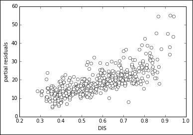
For the specific problem of detecting non-linearity, we are going to use a plot based on residuals called the partial residual plot. In this plot, we compare the regression residuals summed with the values derived from the modeled coefficient of a variable against the original values of the variable itself:
In: var = 7 # the variable in position 7 is DIS
  partial_residual = residuals + X[:,var] * linear_regression.coef_[var]
  plt.plot(X[:,var], partial_residual, 'wo')
  plt.xlabel(boston.feature_names[var])
  plt.ylabel('partial residuals')
  plt.show()
Out:

After having calculated the residual of the regression, we decide to inspect one variable at a time. After picking up our selected variable, we create a partial residual by summing the residuals of the regression with the multiplication of the variable values multiplied by its coefficient. In such a way, we extract the variable from the regression line and we put it in the residuals. Now, as partial residuals, we have both the errors and the coefficient-weighted variable. If we plot it against the variable itself, we can notice whether there is any non-linear pattern. If there is one, we know that we should try some modification.
In our case, there is some sign that the points bend after the value 2 of our variable, a clear non-linearity sign such as any bend or pattern different from an elongated, straight cloud of points. Square, inverse, logarithmic transformations can often solve such problems without adding new terms, such as when using the polynomial expansion:
In: X_t = X.copy()
  X_t[:,var] = 1./np.sqrt(X_t[:,var])
  linear_regression.fit(X_t, y)
  partial_residual = residuals + X_t[:,var] * linear_regression.coef_[var]
  plt.plot(X_t[:,var], partial_residual, 'wo')
  plt.xlabel(boston.feature_names[var])
  plt.ylabel('partial residuals')
  plt.show()
  print ("R-squared: %0.3f" % r2_score(y, linear_regression.predict(X_t)))

Out: R-squared: 0.769
Just notice how an inverse square transformation rendered the partial residual plot straighter, something that is reflected in a higher R-squared value, indicating an increased capacity of the model to capture the data distribution.
As a rule, the following transformations should always be tried (singularly or in combination) to find a fix for a non-linearity:
|
Function names |
Functions |
|---|---|
|
Logarithmic |
|
|
Exponential |
|
|
Squared |
|
|
Cubed |
|
|
Square root |
|
|
Cube root |
|
|
Inverse |
|
Tip
Some of the transformations suggested in the preceding table won't work properly after normalization or otherwise in the presence of zero and negative values: logarithmic transformation needs positive values above zero, square root won't work with negative values, and inverse transformation won't operate with zero values. Sometimes adding a constant may help (like in the case of np.log(x+1)). Generally, just try the possible transformations, according to your data values.
When it is not easy to figure out the exact transformation, a quick solution could be to transform the continuous numeric variable into a series of binary variables, thus allowing the estimation of a coefficient for each single part of the numeric range of the variable.
Though fast and convenient, this solution will increase the size of your dataset (unless you use a sparse representation of the matrix) and it will risk too much overfitting on your data.
First, you divide your values into equally spaced bins and you notice the edges of the bins using the histogram function from Numpy. After that, using the digitize function, you convert the value in their bin number, based on the bin boundaries provided before. Finally, you can transform all the bin numbers into binary variables using the previously present LabelBinarizer from Scikit-learn.
At this point, all you have to do is replace the previous variable with this new set of binary indicators and refit the model for checking the improvement:
In: import numpy as np
  from sklearn.preprocessing import LabelBinarizer
  LB = LabelBinarizer()
  X_t = X.copy()
  edges = np.histogram(X_t[:,var], bins=20)[1]
  binning = np.digitize(X_t[:,var], edges)
  X_t = np.column_stack((np.delete(X_t, var, axis=1),LB.fit_transform(binning)))
  linear_regression.fit(X_t, y)
  print ("R-squared: %0.3f" % r2_score(y, linear_regression.predict(X_t)))

Out: R-squared: 0.768