
The last problem we're going to see in this chapter is about prediction in time. The standard name for these problems is time series analysis, since the prediction is made on descriptors extracted in the past; therefore, the outcome at the current time will become a feature for the prediction of the next point in time. In this exercise, we're using the closing values for several stocks composing the Dow Jones index in 2011.
Several features compose the dataset, but in this problem (to make a short and complete exercise) we're just using the closing values of each week for each of the 30 measured stocks, ordered in time. The dataset spans six months: we're using the first half of the dataset (corresponding to the first quarter of the year under observation, with 12 weeks) to train our algorithm, and the second half (containing the second quarter of the year, with 13 weeks) to test the predictions.
Moreover, since we don't expect readers to have a background in economics, we've tried to make things as simple as possible. In a real-life situation, such a prediction will be too simple to get money out of the market, but in this short example we've tried to keep the focus on the time series analysis, dropping all the other inputs and sources.
Note
The full description of this problem can be found at: https://archive.ics.uci.edu/ml/datasets/Dow+Jones+Index.
According to the readme file distributed along with the dataset, there are no missing values; therefore, the loading operation is quite straightforward:
In:
import matplotlib.pyplot as plt
%matplotlib inline

import numpy as np
import pandas as pd

dataset = pd.read_csv('./dji/dow_jones_index.data')
Let's now try to decode the rows we're interested in (stock and close): it seems that the closing values are all strings, starting with $ and followed by the floating point value relative to the closing price. We should then select the correct columns and cast the closing price to the right data type:
In:
print(dataset.head())
Out:
   quarter stock       date    open    high     low   close     volume
0        1    AA   1/7/2011  $15.82  $16.72  $15.78  $16.42  239655616
1        1    AA  1/14/2011  $16.71  $16.71  $15.64  $15.97  242963398
2        1    AA  1/21/2011  $16.19  $16.38  $15.60  $15.79  138428495
3        1    AA  1/28/2011  $15.87  $16.63  $15.82  $16.13  151379173
4        1    AA   2/4/2011  $16.18  $17.39  $16.18  $17.14  154387761

   percent_change_price  percent_change_volume_over_last_wk
0               3.79267                                 NaN
1              -4.42849                            1.380223
2              -2.47066                          -43.024959
3               1.63831                            9.355500
4               5.93325                            1.987452

   previous_weeks_volume next_weeks_open next_weeks_close
0                    NaN          $16.71           $15.97
1              239655616          $16.19           $15.79
2              242963398          $15.87           $16.13
3              138428495          $16.18           $17.14
4              151379173          $17.33           $17.37

   percent_change_next_weeks_price  days_to_next_dividend
0                        -4.428490                     26
1                        -2.470660                     19
2                         1.638310                     12
3                         5.933250                      5
4                         0.230814                     97

   percent_return_next_dividend
0                      0.182704
1                      0.187852
2                      0.189994
3                      0.185989
4                      0.175029
In:
observations = {}

for el in dataset[['stock', 'close']].iterrows():

    stock = el[1].stock
    close = float(el[1].close.replace("$", ""))

    try:
        observations[stock].append(close)
    except KeyError:
        observations[stock] = [close]
Let's now create a feature vector for each stock. In the simplest instance, it's just a row containing the sorted closing prices for the 25 weeks:
In:
X = []
stock_names = sorted(observations.keys())

for stock in stock_names:
    X.append(observations[stock])

X = np.array(X)
Let's now build a baseline: we can try the regressor on the first 12 weeks, and then test it by recursively offsetting the data—that is, to predict the 13th week, we use the first 12 weeks; to predict the value at the 14th week, we use 12 weeks ending with the 13th one. And so on.
Note that, in this very simple approach, we build just a classifier for all the stocks, independently by their price, and we use both R2 and MAE to score our learner for each week of analysis (a score for the 13th week, one for the 14th, and so on). Finally, we compute mean and variance of these scores:
In:
from sklearn.linear_model import LinearRegression
from sklearn.metrics import r2_score, mean_absolute_error

X_train = X[:, :12]
y_train = X[:, 12]

regr_1 = LinearRegression()
regr_1.fit(X_train, y_train)
In:
plot_vals = []

for offset in range(0, X.shape[1]-X_train.shape[1]):
    X_test = X[:, offset:12+offset]
    y_test = X[:, 12+offset]

    r2 = r2_score(y_test, regr_1.predict(X_test))
    mae = mean_absolute_error(y_test, regr_1.predict(X_test))

    print("offset=", offset, "r2_score=", r2)
    print("offset=", offset, "MAE     =", mae)

    plot_vals.append( (offset, r2, mae) )

print()
print("r2_score: mean=", np.mean([x[1] for x in plot_vals]), "variance=", np.var([x[1] for x in plot_vals]))
print("mae_score: mean=", np.mean([x[2] for x in plot_vals]), "variance=", np.var([x[2] for x in plot_vals]))
Out:
offset= 0 r2_score= 0.999813479679
offset= 0 MAE     = 0.384145971072
offset= 1 r2_score= 0.99504246854
offset= 1 MAE     = 1.602203752
offset= 2 r2_score= 0.995188278161
offset= 2 MAE     = 1.76248455475
offset= 3 r2_score= 0.998287091734
offset= 3 MAE     = 1.15856848271
offset= 4 r2_score= 0.997938802118
offset= 4 MAE     = 1.11955148717
offset= 5 r2_score= 0.985036566148
offset= 5 MAE     = 2.94239117688
offset= 6 r2_score= 0.991598279578
offset= 6 MAE     = 2.35632383083
offset= 7 r2_score= 0.995485519307
offset= 7 MAE     = 1.73191962456
offset= 8 r2_score= 0.992872581249
offset= 8 MAE     = 1.9828644662
offset= 9 r2_score= 0.990012202362
offset= 9 MAE     = 2.66825249081
offset= 10 r2_score= 0.996984329367
offset= 10 MAE     = 1.38682132207
offset= 11 r2_score= 0.999029861989
offset= 11 MAE     = 0.761720947323
offset= 12 r2_score= 0.996280599178
offset= 12 MAE     = 1.53124828142

r2_score: mean= 0.99489000457 variance= 1.5753065199e-05
mae_score: mean= 1.64526895291 variance= 0.487371842069
On the 13 testing weeks, the R2 is 0.99 on average (with a variance of 0.0000157) and the MAE is 1.64 on average (with a variance of 0.48). That's the baseline; let's plot it:
In:
fig, ax1 = plt.subplots()
ax1.plot([x[0] for x in plot_vals], [x[1] for x in plot_vals], 'b-')
ax1.plot(plot_vals[0][0], plot_vals[0][1], 'bo')

ax1.set_xlabel('test week')
# Make the y-axis label and tick labels match the line color.
ax1.set_ylabel('r2_score', color='b')
for tl in ax1.get_yticklabels():
    tl.set_color('b')
ax1.set_ylim([0.9, 1.1])


ax2 = ax1.twinx()
ax2.plot([x[0] for x in plot_vals], [x[2] for x in plot_vals], 'r-')
ax2.plot(plot_vals[0][0], plot_vals[0][2], 'ro')
ax2.set_ylabel('mae score', color='r')
for tl in ax2.get_yticklabels():
    tl.set_color('r')
ax2.set_ylim([0, 3.3])

plt.xlim([-.1, 12.1])

plt.show()
Out: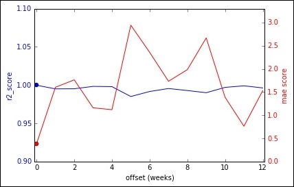
Are we sure that the value of 12 weeks ago is still a good predictor for the current week? Let's now try to improve our scores by decreasing the training weeks. As an additional advantage, we will also have more training data. Let's try using 5 (a little more than a month):
In:
training_len = 5

X_train_short = X[:, :training_len]
y_train_short = X[:, training_len]


for offset in range(1, 12-training_len):
    X_train_short = np.vstack( (X_train_short, X[:, offset:training_len+offset]) )
    y_train_short = np.concatenate( (y_train_short, X[:, training_len+offset]) )
In:
regr_2 = LinearRegression()
regr_2.fit(X_train_short, y_train_short)
In:
plot_vals = []

for offset in range(0, X.shape[1]-X_train.shape[1]):
    X_test = X[:, 12-training_len+offset:12+offset]
    y_test = X[:, 12+offset]

    r2 = r2_score(y_test, regr_2.predict(X_test))
    mae = mean_absolute_error(y_test, regr_2.predict(X_test))

    print("offset=", offset, "r2_score=", r2)
    print("offset=", offset, "MAE     =", mae)

    plot_vals.append( (offset, r2, mae) )

print()
print("r2_score: mean=", np.mean([x[1] for x in plot_vals]), "variance=", np.var([x[1] for x in plot_vals]))
print("mae_score: mean=", np.mean([x[2] for x in plot_vals]), "variance=", np.var([x[2] for x in plot_vals]))
Out:
offset= 0 r2_score= 0.998579501272
offset= 0 MAE     = 0.85687189133
offset= 1 r2_score= 0.999412004606
offset= 1 MAE     = 0.552138850961
offset= 2 r2_score= 0.998668959234
offset= 2 MAE     = 0.941052814674
offset= 3 r2_score= 0.998291291965
offset= 3 MAE     = 1.03476245234
offset= 4 r2_score= 0.997006831124
offset= 4 MAE     = 1.45857426198
offset= 5 r2_score= 0.996849578723
offset= 5 MAE     = 1.04394939395
offset= 6 r2_score= 0.998134003499
offset= 6 MAE     = 1.05938998285
offset= 7 r2_score= 0.998391605331
offset= 7 MAE     = 0.865007491822
offset= 8 r2_score= 0.999317752361
offset= 8 MAE     = 0.607975744054
offset= 9 r2_score= 0.996058731277
offset= 9 MAE     = 1.62548930127
offset= 10 r2_score= 0.997319345983
offset= 10 MAE     = 1.2305378204
offset= 11 r2_score= 0.999264102166
offset= 11 MAE     = 0.649407612032
offset= 12 r2_score= 0.998227164258
offset= 12 MAE     = 1.020568135

r2_score: mean= 0.998116990138 variance= 9.8330905525e-07
mae_score: mean= 0.995825057897 variance= 0.0908384278533
With this approach, both R2 and MAE have improved, on average, and their variance is perceptibly lower:
In:
fig, ax1 = plt.subplots()
ax1.plot([x[0] for x in plot_vals], [x[1] for x in plot_vals], 'b-')
ax1.plot(plot_vals[0][0], plot_vals[0][1], 'bo')

ax1.set_xlabel('test week')
# Make the y-axis label and tick labels match the line color.
ax1.set_ylabel('r2_score', color='b')
for tl in ax1.get_yticklabels():
    tl.set_color('b')
ax1.set_ylim([0.95, 1.05])


ax2 = ax1.twinx()
ax2.plot([x[0] for x in plot_vals], [x[2] for x in plot_vals], 'r-')
ax2.plot(plot_vals[0][0], plot_vals[0][2], 'ro')
ax2.set_ylabel('mae score', color='r')
for tl in ax2.get_yticklabels():
    tl.set_color('r')
ax2.set_ylim([0, 2.2])

plt.xlim([-.1, 12.1])

plt.show()
Out:
Since the approach seems to be working better, let's now try to grid-search the best training length, spanning from 1 to 12:
In:
training_lens = range(1,13)
models = {}


for training_len in training_lens:
    X_train_short = X[:, :training_len]
    y_train_short = X[:, training_len]

    for offset in range(1, 12-training_len):
        X_train_short = np.vstack( (X_train_short, X[:, offset:training_len+offset]) )
        y_train_short = np.concatenate( (y_train_short, X[:, training_len+offset]) )

    regr_x = LinearRegression()
    regr_x.fit(X_train_short, y_train_short)
    models[training_len] = regr_x

    plot_vals = []

    for offset in range(0, X.shape[1]-X_train.shape[1]):
        X_test = X[:, 12-training_len+offset:12+offset]
        y_test = X[:, 12+offset]

        r2 = r2_score(y_test, regr_x.predict(X_test))
        mae = mean_absolute_error(y_test, regr_x.predict(X_test))

        plot_vals.append( (offset, r2, mae) )

    fig, ax1 = plt.subplots()
    ax1.plot([x[0] for x in plot_vals], [x[1] for x in plot_vals], 'b-')
    ax1.plot(plot_vals[0][0], plot_vals[0][1], 'bo')

    ax1.set_xlabel('test week')
    # Make the y-axis label and tick labels match the line color.
    ax1.set_ylabel('r2_score', color='b')
    for tl in ax1.get_yticklabels():
        tl.set_color('b')
    ax1.set_ylim([0.95, 1.05])


    ax2 = ax1.twinx()
    ax2.plot([x[0] for x in plot_vals], [x[2] for x in plot_vals], 'r-')
    ax2.plot(plot_vals[0][0], plot_vals[0][2], 'ro')
    ax2.set_ylabel('mae score', color='r')
    for tl in ax2.get_yticklabels():
        tl.set_color('r')
    ax2.set_ylim([0, max([2.2, 1.1*np.max([x[2] for x in plot_vals])])])

    plt.xlim([-.1, 12.1])

    plt.title("results with training_len={}".format(training_len))

    plt.show()

    print("r2_score: mean=", np.mean([x[1] for x in plot_vals]), "variance=", np.var([x[1] for x in plot_vals]))
    print("mae_score: mean=", np.mean([x[2] for x in plot_vals]), "variance=", np.var([x[2] for x in plot_vals]))

Out:
... [images are omitted] ...
results with training_len=1
r2_score: mean= 0.998224065712 variance= 1.00685934679e-06
mae_score: mean= 0.95962574798 variance= 0.0663013566722

results with training_len=2
r2_score: mean= 0.998198628321 variance= 9.17757825917e-07
mae_score: mean= 0.969741651259 variance= 0.0661101843822

results with training_len=3
r2_score: mean= 0.998223327997 variance= 8.57207677825e-07
mae_score: mean= 0.969261583196 variance= 0.0715715354908

results with training_len=4
r2_score: mean= 0.998223602314 variance= 7.91949263056e-07
mae_score: mean= 0.972853132744 variance= 0.0737436496017

results with training_len=5
r2_score: mean= 0.998116990138 variance= 9.8330905525e-07
mae_score: mean= 0.995825057897 variance= 0.0908384278533

results with training_len=6
r2_score: mean= 0.997953763986 variance= 1.14333232014e-06
mae_score: mean= 1.04107069762 variance= 0.100961792252

results with training_len=7
r2_score: mean= 0.997481850128 variance= 1.85277659214e-06
mae_score: mean= 1.19114613181 variance= 0.121982635728

results with training_len=8
r2_score: mean= 0.99715522262 variance= 3.27488548806e-06
mae_score: mean= 1.23998671525 variance= 0.173529737205

results with training_len=9
r2_score: mean= 0.995975415477 variance= 5.76973840581e-06
mae_score: mean= 1.48200981286 variance= 0.22134177338

results with training_len=10
r2_score: mean= 0.995828230003 variance= 4.92217626753e-06
mae_score: mean= 1.51007677609 variance= 0.209938740518

results with training_len=11
r2_score: mean= 0.994520917305 variance= 7.24129427869e-06
mae_score: mean= 1.78424593989 variance= 0.213259808552

results with training_len=12
r2_score: mean= 0.99489000457 variance= 1.5753065199e-05
mae_score: mean= 1.64526895291 variance= 0.487371842069
The best trade-off is with training_len=3.
As you've seen, in this example we didn't normalize the data, using stocks with high and low prices together. This fact may confuse the learner, since the observations don't have the same center. With a bit of preprocessing, we may obtain better results, applying a per-stock normalization. Can you think what else could we do, and how could we test the algorithm?