
In the previous chapter, we introduced linear regression as a supervised method for machine learning rooted in statistics. Such a method forecasts numeric values using a combination of predictors, which can be continuous numeric values or binary variables, given the assumption that the data we have at hand displays a certain relation (a linear one, measurable by a correlation) with the target variable. To smoothly introduce many concepts and easily explain how the method works, we limited our example models to just a single predictor variable, leaving to it all the burden of modeling the response.
However, in real-world applications, there may be some very important causes determining the events you want to model but it is indeed rare that a single variable could take the stage alone and make a working predictive model. The world is complex (and indeed interrelated in a mix of causes and effects) and often it cannot be easily explained without considering various causes, influencers, and hints. Usually more variables have to work together to achieve better and reliable results from a prediction.
Such an intuition decisively affects the complexity of our model, which from this point forth will no longer be easily represented on a two-dimensional plot. Given multiple predictors, each of them will constitute a dimension of its own and we will have to consider that our predictors are not just related to the response but also related among themselves (sometimes very strictly), a characteristic of data called multicollinearity.
Before starting, we'd like to write just a few words on the selection of topics we are going to deal with. Though in the statistical literature there is a large number of publications and books devoted to regression assumptions and diagnostics, you'll hardly find anything here because we will leave out such topics. We will be limiting ourselves to discussing problems and aspects that could affect the results of a regression model, on the basis of a practical data science approach, not a purely statistical one.
Given such premises, in this chapter we are going to:
- Extend the procedures for a single regression to a multiple one, keeping an eye on possible sources of trouble such as multicollinearity
- Understand the importance of each term in your linear model equation
- Make your variables work together and increase your ability to predict using interactions between variables
- Leverage polynomial expansions to increase the fit of your linear model with non-linear functions
To recap the tools seen in the previous chapter, we reload all the packages and the Boston dataset:
In: import numpy as np
  import pandas as pd
  import matplotlib.pyplot as plt
  import matplotlib as mpl
  from sklearn.datasets import load_boston
  from sklearn import linear_model
If you are working on the code in an IPython Notebook (as we strongly suggest), the following magic command will allow you to visualize plots directly on the interface:
In: %matplotlib inline
We are still using the Boston dataset, a dataset that tries to explain different house prices in the Boston of the 70s, given a series of statistics aggregated at the census zone level:
In: boston = load_boston()
  dataset = pd.DataFrame(boston.data, columns=boston.feature_names)
  dataset['target'] = boston.target
We will always work by keeping with us a series of informative variables, the number of observation and variable names, the input data matrix, and the response vector at hand:
In: observations = len(dataset)
  variables = dataset.columns[:-1]
  X = dataset.ix[:,:-1]
  y = dataset['target'].values
As a first step toward extending to more predictors the previously done analysis with Statsmodels, let's reload the necessary modules from the package (one working with matrices and the other with formulas) :
In: import statsmodels.api as sm
  import statsmodels.formula.api as smf
Let's also prepare a suitable input matrix, naming it Xc after having it incremented by an extra column containing the bias vector (a constant variable having the unit value):
In: Xc = sm.add_constant(X)
  linear_regression = sm.OLS(y,Xc)
  fitted_model = linear_regression.fit()
After having fitted the preceding specified model, let's immediately ask for a summary:
In: fitted_model.summary()
Out:
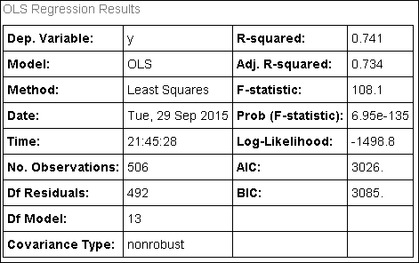


Basically, the enunciations of the various statistical measures, as presented in the previous chapter, are still valid. We will just devote a few words to remarking on a couple of extra features we couldn't mention before because they are related to the presence of multiple predictors.
First, the adjusted R-squared is something to take note of now. When working with multiple variables, the standard R-squared can get inflated because of the many coefficients inserted into the model. If you are using too many predictors, its measure will diverge perceptibly from the plain R-squared. The adjusted R-squared considers the complexity of the model and reports a much more realistic R-squared measure.
This is not the case in our example because the difference is quite slight, approximately between 0.741 and 0.734, which translated into a ratio turns out to be 0.741/0.734 = 1.01, that is just 1% over the standard R-squared.
Then, working with so many variables at a time, coefficients should also be checked for important warnings. The risk involved is having coefficients picking up noisy and non-valuable information. Usually such coefficients will not be far from zero and will be noticeable because of their large standard errors. Statistical t-tests are the right tool to spot them.
In our example, being largely not significant (p-value major of 0.05), the AGE and INDUS variables are represented in the model by coefficients whose usefulness could be seriously challenged.
Finally, the condition number test (Cond. No.) is another previously mentioned statistic that now acquires a fresh importance under the light of a system of predictors. It signals numeric unstable results when trying an optimization based on matrix inversion. The cause of such instability is due to multicollinearity, a problem we are going to expand on in the following paragraphs.
Tip
When a condition number is over the score of 30, there's a clear signal that unstable results are rendering the result less reliable. Predictions may be affected by errors and the coefficients may drastically change when rerunning the same regression analysis with a subset or a different set of observations.
In our case, the condition number is well over 30, and that's a serious warning signal.
To obtain the same results using the statsmodels.formula.api and thereby explicating a formula to be interpreted by the Patsy package (http://patsy.readthedocs.org/en/latest/), we use:
linear_regression = smf.ols(formula = 'target ~ CRIM + ZN +INDUS + CHAS + NOX + RM + AGE + DIS + RAD + TAX + PTRATIO + B + LSTAT', data=dataset)
fitted_model = linear_regression.fit()
In this case, you have to explicate all the variables to enter into model building by naming them on the right side of the formula. After fitting the model, you can use all the previously seen Statsmodels methods for reporting the coefficients and results.
When trying to model the response using a single predictor, we used Pearson's correlation (Pearson was the name of its inventor) to estimate a coefficient of linear association between the predictor and the target. Having more variables in the analysis now, we are still quite interested in how each predictor relates to the response; however, we have to distinguish whether the relation between the variance of the predictor and that of the target is due to unique or shared variance.
The measurement of the association due to unique variance is called partial correlation and it expresses what can be guessed of the response thanks to the information uniquely present in a variable. It represents the exclusive contribution of a variable in predicting the response, its unique impact as a direct cause to the target (if you can view it as being a cause though, because, as seen, correlation is not causation).
The shared variance is instead the amount of information that is simultaneously present in a variable and in other variables in the dataset at hand. Shared variance can have many causes; maybe one variable causes or it just interferes with the other (as we described in the previous chapter in the Correlation is not causation section ). Shared variance, otherwise called collinearity (between two variables) or multicollinearity (among three or more variables), has an important effect, worrisome for the classical statistical approach, less menacing for the data science one.
For the statistical approach, it has to be said that high or near perfect multicollinearity not only often renders coefficient estimations impossible (matrix inversion is not working), but also, when it is feasible, it will be affected by imprecision in coefficient estimation, leading to large standard errors of the coefficients. However, the predictions won't be affected in any way and that leads us to the data science points of view.
Having multicollinear variables, in fact, renders it difficult to select the correct variables for the analysis (since the variance is shared, it is difficult to figure out which variable should be its causal source), leading to sub-optimal solutions that could be resolved only by augmenting the number of observations involved in the analysis.
To determine the manner and number of predictors affecting each other, the right tool is a correlation matrix, which, though a bit difficult to read when the number of the features is high, is still the most direct way to ascertain the presence of shared variance:
X = dataset.ix[:,:-1]
correlation_matrix = X.corr()
print (correlation_matrix)
This will give the following output:

At first glance, some high correlations appear to be present in the order of the absolute value of 0.70 (highlighted by hand in the matrix) between TAX, NOX, INDUS, and DIS. That's fairly explainable since DIS is the distance from employment centers, NOX is a pollution indicator, INDUS is the quota of non-residential or commercial buildings in the area, and TAX is the property tax rate. The right combination of these variables can well hint at what the productive areas are.
A faster, but less numerical representation is to build a heat map of the correlations:
In:
def visualize_correlation_matrix(data, hurdle = 0.0):
    R = np.corrcoef(data, rowvar=0)
    R[np.where(np.abs(R)<hurdle)] = 0.0
    heatmap = plt.pcolor(R, cmap=mpl.cm.coolwarm, alpha=0.8)
    heatmap.axes.set_frame_on(False)
    heatmap.axes.set_yticks(np.arange(R.shape[0]) + 0.5, minor=False)
    heatmap.axes.set_xticks(np.arange(R.shape[1]) + 0.5, minor=False)
    heatmap.axes.set_xticklabels(variables, minor=False)
    plt.xticks(rotation=90)
    heatmap.axes.set_yticklabels(variables, minor=False)
    plt.tick_params(axis='both', which='both', bottom='off', 	op='off', left = 'off', right = 'off')
    plt.colorbar()
    plt.show()

visualize_correlation_matrix(X, hurdle=0.5)
This will give the following output:

Having a cut at 0.5 correlation (which translates into a 25% shared variance), the heat map immediately reveals how PTRATIO and B are not so related to other predictors. As a reminder of the meaning of variables, B is an indicator quantifying the proportion of colored people in the area and PTRATIO is the pupil-teacher ratio in the schools of the area. Another intuition provided by the map is that a cluster of variables, namely TAX, INDUS, NOX, and RAD, is confirmed to be in strong linear association.
An even more automatic way to detect such associations (and figure out numerical problems in a matrix inversion) is to use eigenvectors. Explained in layman's terms, eigenvectors are a very smart way to recombine the variance among the variables, creating new features accumulating all the shared variance. Such recombination can be achieved using the NumPy linalg.eig function, resulting in a vector of eigenvalues (representing the amount of recombined variance for each new variable) and eigenvectors (a matrix telling us how the new variables relate to the old ones):
In: corr = np.corrcoef(X, rowvar=0)
  eigenvalues, eigenvectors = np.linalg.eig(corr)
After extracting the eigenvalues, we print them in descending order and look for any element whose value is near to zero or small compared to the others. Near zero values can represent a real problem for normal equations and other optimization methods based on matrix inversion. Small values represent a high but not critical source of multicollinearity. If you spot any of these low values, keep a note of their index in the list (Python indexes start from zero).
In: print (eigenvalues)
Out: [ 6.12265476  1.43206335  1.24116299  0.85779892  0.83456618  0.65965056  0.53901749  0.39654415  0.06351553  0.27743495  0.16916744  0.18616388  0.22025981]
Using their index position in the list of eigenvalues, you can recall their specific vector from eigenvectors, which contains all the variable loadings—that is, the level of association with the original variables. In our example, we investigate the eigenvector at index 8. Inside the eigenvector, we notice values at index positions 2, 8, and 9, which are indeed outstanding in terms of absolute value:
In: print (eigenvectors[:,8])
Out: [-0.04552843  0.08089873  0.25126664 -0.03590431 -0.04389033 -0.04580522  0.03870705  0.01828389  0.63337285 -0.72024335 -0.02350903  0.00485021 -0.02477196]
We now print the variables' names to know which ones contribute so much by their values to build the eigenvector:
In: print (variables[2], variables[8], variables[9])
Out: INDUS RAD TAX
Having found the multicollinearity culprits, what remedy could we use for such variables? Removal of some of them is usually the best solution and that will be carried out in an automated way when exploring how variable selection works in Chapter 6, Achieving Generalization.