1
The Fractional Integrator
1.1. Introduction
A fundamental topic of mathematics concerns the integration of ordinary differential equations (ODEs). Except particular cases where analytical solutions exist, the search for general solutions for any type of ODE and excitation has been an important issue either theoretically or numerically for engineering applications. The quest for practical solutions has motivated the formulation of approximate numerical solutions (Euler, Runge–Kutta, etc.) and the realization of mechanical and electrical computers based on a physical analogy. The interest of an historical reminder concerning analog computers is to highlight the fundamental role played by the integration operator, which is also present in an implicit form in numerical ODE solvers.
As in the integer order case, the integration of fractional differential equations (FDEs) requires a fractional integration operator, which is the topic of this chapter. After a reminder of the integer order ODE simulation, the Riemann–Liouville integration or fractional order integration is presented as a generalization of repeated integer order integration. Then, the fractional integration operator is defined and applied to the FDE simulation. The realization of the fractional integrator will be addressed in Chapter 2.
1.2. Simulation and modeling of integer order ordinary differential equations
1.2.1. Simulation with analog computers
Analog computers are nowadays obsolete, but they present a fundamental interest: they exhibit the key role played by integrators in simulation. According to the principle formulated by Lord Kelvin [THO 76] (see Appendix A.1.1), only integrators are required to simulate an ODE. This principle has been used in analog computers, i.e. mechanical computers from 1931 to 1945 and electronic computers from 1945 to 1970 (see Appendix A.1.2).
Some analog computers are still used in electronics and automatic control education. It is important to note that the only active operator proposed to the user is the integrator, in association with adders, multipliers and so on, but with no differentiation operator! Of course, there is a fundamental reason: it is well known that the amplification of a differentiator increases with frequency. Therefore, the noise, characterized by a wide frequency spectrum, is amplified and saturates the operator output. Thus, the first paradox is that differentiators cannot be used to simulate ODEs! In fact, derivatives should not be used explicitly.
In order to avoid explicit differentiation, analog computers use the integrator property:
and reciprocally:
where v(t) is defined as the implicit derivative of x(t) . Note that this property does not allow the computation of ![]() in an open-loop operation. On the contrary, with the closed-loop diagram of Figure 1.1, used to simulate:
in an open-loop operation. On the contrary, with the closed-loop diagram of Figure 1.1, used to simulate:

Figure 1.1. Analog simulation of one-derivative ODE
the signal v(t) is defined as
Therefore, v(t) , input of the integrator, represents the derivative of the solution x(t) , without explicit calculation of this derivative.
1.2.2. Simulation with digital computers
Obviously, analog computers are no longer used to simulate ODEs. Therefore, we may ask the question: is Lord Kelvin’s principle really used with digital computers and numerical algorithms?
Consider the previous ODE and Euler’s technique, based on the explicit definition of the derivative:
The corresponding algorithm is:
This algorithm is based on the explicit definition of the derivative; so where is the integrator? It is straightforward to write:
which corresponds to (using the delay operator q-1):
Hence, xk is the numerical integral of vk: it means that integrator ![]() of Figure 1.1 has been replaced by a numerical integrator:
of Figure 1.1 has been replaced by a numerical integrator:
Therefore, whatever can be the numerical algorithm used to simulate the ODE, it is possible to demonstrate that it corresponds to a sophisticated numerical integrator (see, for example, Appendix A.1.3 for the interpretation of the RK2 algorithm). We can conclude that the simulation of ODEs is based essentially on integrators. Moreover, explicit differentiation is carefully avoided. If necessary, the input of the integrator provides the implicit derivative.
1.2.3. Initial conditions
The initial condition problem is elementary in the integer order case; on the contrary, it is complex in the fractional order case. It is the reason why we insist on certain points that will facilitate the generalization of the methodology to the simulation of FDSs/FDEs. Therefore, consider the electronic integrator of Figure 1.2.
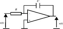
Figure 1.2. Analog realization of the integer order integrator
It is well known that:
Moreover, x(t) is equal to the voltage at C terminals.
Hence, if the capacitor is initially charged at t = 0 :
Therefore, x(0), the initial condition of the integrator, is not only an abstract mathematical value but also a physical phenomenon. Moreover, it is linked to the initial energy of the integrator since:
EC(t) represents the electrostatic energy stored in the capacitor. It can also be interpreted as the Lyapunov function of the integrator, and thus of system [1.3]. Practically, this energy is expressed as:
REMARK 1.– Energy issues, particularly in relation to fractional order systems, are analyzed in Chapter 7 Volume 2.
Note that x(0) only concerns the output of the integrator and is not related to its derivative ![]() .
.
Consider Laplace transform of [1.1]:
As ![]() , we can write:
, we can write:
which is known as the Laplace transform of the derivative: usually, x(0) is considered as the initial condition of the derivative. Of course, an integer order derivative has no initial condition; x(0) is in fact the initial condition of the associated integrator. This remark is essential with the fractional integrator.
1.2.4. State space representation and simulation diagram
A state space representation is not specific to automatic control and system theory. It has long been used in mathematics and mechanics (see, for example, the phase plane technique and limit cycles of Poincaré [POI 82]). However, the simulation diagrams used on analog computers refer explicitly to state space equations. It is certainly one of the reasons of the emergence of state space theory in the 1950s, in parallel with the development of analog computing for the simulation of automatic control systems [LEV 64]. Moreover, the first monographs [DOR 67, WIB 71, FRI 86] on state space theory referred explicitly to flow diagrams, which are the simulation diagrams, exhibiting integrators and their initial conditions.
Consider, for example, the two-derivative ODE:
which requires two integrators for its simulation (see Figure 1.3).

Figure 1.3. Analog simulation of a two-derivative ODE
This diagram can be replaced by a state space representation, with ![]() and
and ![]() .
.
Then:
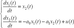
corresponds to the well-known model:
with
This connection between simulation/flow diagrams and state space models is well recalled in Kailath [KAI 80], who insists on the physical meaning of initial conditions and our tribute to Lord Kelvin’s principle.
Using Laplace transform, the solution of the differential system is:
where x(0) is the initial state of [1.17], i.e. of the different integrators. The first term represents the free response, i.e. the initialization of the differential system.
REMARK 2.– State is related to energy, as mentioned previously. It is also defined as the essential information required to predict the future system behavior. Therefore, we have to recall that state definition and system initialization are coupled problems.
REMARK 3.– Equation [1.18] is interesting because it is a compact writing of flow diagrams. On the contrary, it represents some risk because it does not refer to integrators which are implicit. Of course, there is no risk of confusion with integer order differential systems. However, direct generalization of equation [1.18] to fractional order systems, without reference to the characteristics of their specific integrators, has certainly led to questionable definitions of fractional state variables.
REMARK 4.– The simulation diagram presented in Figure 1.3 is a closed-loop system: it is a closed-loop representation of system [1.16]. As with any closed-loop system, its stability is conditional: of course, its stability condition is the same as that of the ODE [1.18]. An elementary modification of this diagram shows that its stability can be analyzed using the Nyquist criterion [NYQ 32]: this approach gives the same results as the Routh criterion [ROU 77], with the advantage of stability margins, giving indications on the stability degree of the ODE. This methodology is presented in Chapter 6 Volume 2. It has been published in [TRI 09c] and generalized to the stability of FDEs and time delay systems [MAA 09].
1.2.5. Concluding remarks
The interest of this reminder has been to insist on some fundamental principles which will be generalized to fractional differential systems (FDSs):
– only integrators are required for the simulation of ODEs;
- – integrators perform the integrals:
 ;
; - – vi(t) is the implicit derivative of
 ;
; - – xi(0) is the initial condition of the ith integrator; it corresponds to the initial charge of capacitor Ci for an analog integrator, i.e. its initial energy;
- – the state variables xi(t) are the outputs of the different integrators; explicit differentiation is not required for the simulation of ODEs.
1.3. Origin of fractional integration: repeated integration
We can define the fractional integration of the order n (n real) or the Riemann–Liouville integration using the repeated integration of the order N (N integer) [MAT 94, POD 99].
Let f(τ) be a function defined for τ ≥ 0.
Moreover, let us define
I1(τ) is a new function, defined for τ ≥ 0 , with I1 (0) = 0 .
Then again, we can define
I2(τ) is a repeated integral, defined for τ ≥ 0, with I2(0) = 0.
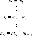
If we continue this repeated integration process until step N, we can define the function IN(τ) with the recursive relation
defined for τ ≥ 0 , with IN(0) = 0 .
Then, let us express IN(t) as a function of f(τ).
Consider the variable change μ = t − τ.
Then
Let us use the integration by parts technique
For N = 2 , we obtain
For N = 3 , a similar procedure provides
Now consider the general case for N repeated integrals:
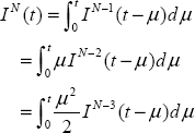
Using i times the integration by parts technique, we obtain
Therefore, for N − 1 − i = 0 or i = N − 1, we obtain
As I0(t − μ) = f(t − μ), we finally obtain the general repeated integration formula
This formula can be interpreted as a convolution between ![]() and f(t), which can be written as
and f(t), which can be written as
Moreover, the function ![]() can be interpreted as the impulse response of a linear filter
can be interpreted as the impulse response of a linear filter
where H(t) is the Heaviside function.
Therefore, we can conclude
1.4. Riemann–Liouville integration
1.4.1. Definition
The Riemann–Liouville integral generalizes the repeated integral for n real thanks to the gamma function Γ(n) which is the interpolation of the factorial function between the integer values of n .
This function Γ(n) (n real) is defined by the integral (see Appendix A.1.4)
Note that (n−1)! = Γ(n) for n integer.
Then, for n real, hn(t) becomes
and the repeated integral IN(t) becomes the fractional integral with order n real (Riemann–Liouville integral) of the function f(t), which we express as [POD 99]:
1.4.2. Laplace transform of the Riemann–Liouville integral
Our objective is to express ![]() .
.
First, we consider
We use the variable change ![]() .
.
Then
As ![]() du , we obtain
du , we obtain
and
As In (f(t)) = hn (t) * f(t), we obtain
Therefore
1.4.3. Fractional integration operator
The case 0 < n < 1 is particularly interesting because it corresponds to the fractional integration operator.
Let us recall that for n = 1, I1(t) corresponds to the integral of f(t):
This integral is provided by the integer order integrator, whose Laplace transform is ![]() . It can be expressed by the diagram of Figure 1.4.
. It can be expressed by the diagram of Figure 1.4.
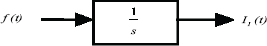
Figure 1.4. Analog simulation of integer order integration
where
If we generalize this relation to 0 < n < 1, the fractional integral In (f(t)) can be interpreted as the diagram of Figure 1.5.

Figure 1.5. Analog simulation of fractional order integration
where ![]() is the fractional integration operator for 0 < n < 1, whose impulse response is hn(t):
is the fractional integration operator for 0 < n < 1, whose impulse response is hn(t):
1.4.4. Fractional differentiation
We can define fractional differentiation as a generalization of integer order differentiation.
Let f(t) be the output of a chain of N integer order integrators ![]() , whose input is
, whose input is ![]() (see Figure 1.6).
(see Figure 1.6).

Figure 1.6. Implicit integer order differentiation
We can write

Therefore
Thus:

Then, if we consider that all the initial conditions are equal to 0, we obtain
Therefore, as a generalization of the previous result for n = N real, if f(t) is the output of the fractional integrator ![]() , its input has to be the nth-order fractional derivative of f(t) : Dn (f(t)) (see Figure 1.7).
, its input has to be the nth-order fractional derivative of f(t) : Dn (f(t)) (see Figure 1.7).

Figure 1.7. Implicit fractional order differentiation
Then
or
Therefore, if the initial conditions are equal to 0 (this complex concept will be defined correctly in Chapter 8), we obtain
Note that sn can be interpreted as
Therefore
and
1.5. Simulation of FDEs with a fractional integrator
1.5.1. Simulation of a one-derivative FDE
Consider the elementary FDE:
We can write:
where v(t) is the input of the fractional integration operator ![]() and x(t) is its output.
and x(t) is its output.

Figure 1.8. Simulation of a FDE
Therefore, the simulation of this FDE is performed as in the integer order case, according to Figure 1.1, where integrator ![]() is replaced by
is replaced by ![]() , which leads to Figure 1.8.
, which leads to Figure 1.8.
1.5.2. FDE
Consider the general linear FDE [POI 03, TRI 09b]:
whose transfer function is:
The fractional differentiation orders:
are real positive numbers; they are called external or explicit orders. It is necessary to define internal or implicit differentiation orders such as:
1.5.3. Simulation of the general linear FDE
Consider the previous FDE [1.59].
Define:
and
which allow the introduction of the classical controller canonical state space form [WIB 71, KAI 80, ZAD 08]:

and

Finally, y(t) is obtained using the relation:
Corresponding to:
This simulation scheme is based on a state space model which requires N fractional integration operators, whose transfer functions are respectively ![]() and connected according to the analog simulation diagram of Figure 1.9, which is the closed-loop representation of system [1.59]. The modeling of FDEs is analyzed in Chapter 7.
and connected according to the analog simulation diagram of Figure 1.9, which is the closed-loop representation of system [1.59]. The modeling of FDEs is analyzed in Chapter 7.

Figure 1.9. Simulation of an FDE with fractional integrators
A.1. Appendix
A.1.1. Lord Kelvin’s principle
Lord Kelvin (Sir W. Thomson) proposed in 1876 [THO 76] a general principle for mechanical integration of the differential equation:
This integration was performed using mechanical integrators, which were connected according to Figure 1.10 (in fact, this figure was proposed by Kailath [KAI 80], who interpreted the original paper).
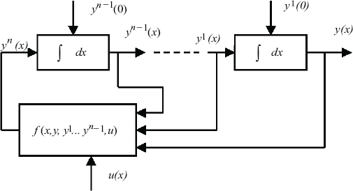
Figure 1.10. Lord Kelvin’s scheme for simulation of the nth-order ODE
Thanks to the principle of mechanical integrators, the independent variable x is not necessarily time t . The main idea is that the chain of integrators avoids the use of differentiators, i.e. the derivatives ![]() are implicit. Although Lord Kelvin can be considered as the father of ODE simulation, he was not able to perform it because friction problems prevented the use of a chain of integrators.
are implicit. Although Lord Kelvin can be considered as the father of ODE simulation, he was not able to perform it because friction problems prevented the use of a chain of integrators.
A.1.2. A brief history of analog computing
A good introduction to the history of analog computing is presented in the special issue of IEEE Control Systems Magazine (June 2005 Volume 25 Number 3) with many references therein.
In 1931, Vannever Bush [OWE 86] of the MIT used Lord Kelvin’s principle and performed the ODE simulation using mechanical integrators. The friction problem was solved by torque amplifiers. This first analog computer was called the differential analyzer. It was regularly improved until the end of World War II. In 1932, D. Hartree (Manchester University G.B.) visited the MIT and proposed a simplified version of the differential analyzer, using Meccano components. Another computer was built in Cambridge University. These first computers were not used for automatic control simulation. In fact, they have been applied to scientific computing, as required by quantum mechanics.
Since 1945, these mechanical computers have been abandoned and replaced by electronic computers, themselves very complex, but more easily duplicated. The heart of these analog computers remained the integrator: it was based on the operational amplifier principle [RAG 47]. The first operational amplifiers, based on a chopper technique, were built with vacuum tubes: they exhibited serious drift problems. An essential improvement was the use of DC differential amplifiers provided by integrated devices in the 1960s. These analog computers have been used in many fields of scientific computing, but particularly for the simulation of automatic control problems arising, for instance, in aeronautics [LEV 64].
Finally, they were supplanted by digital computers and numerical algorithms at the beginning of the 1970s.
A.1.3. Interpretation of the RK2 algorithm
Consider the ODE:
If we know a solution y(t) at the instant t, we can write:
The practical problem is to approximate the integral.
If we use the rectangular rule [HAR 98], we can write:
which corresponds to Euler’s algorithm:
The integral can also be approximated using the trapezoidal rule [HAR 98]:
where f(t + h) is not available at instant t. The curve f(τ,y(τ)) can be approximated by a parabola in the interval [t,t + h]; thus, the mean of ![]() and
and ![]() is equal to
is equal to ![]() .
.
Therefore:
![]() is not available, but it can be approximated by Euler’s algorithm:
is not available, but it can be approximated by Euler’s algorithm:
and finally:
which is known as the Runge–Kutta 2 algorithm [HAR 98] (also known as Heun’s method). Therefore, we can conclude that the RK2 algorithm is equivalent to explicit integration based on the trapezoidal rule.
A.1.4. The gamma function
The gamma function Γ(α) is defined by the integral [ANG 65, POD 99]:
If α is an integer, the gamma function corresponds to the factorial function:
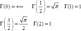
Some important relations:
Integral relation:
Remarkable values: