
7
Modeling of FDEs and FDSs
7.1. Introduction
Chapters 1–3 were dedicated to the numerical simulation of FDEs using fractional integrators. As in the integer order case, the integration operator is the key tool for the modeling of FDSs. In Chapter 6, a theoretical framework was provided to the analysis of this operator. Moreover, it was proved that the Riemann–Liouville integration corresponds basically to a convolution process, obeying the well-known principles of the system theory [KAI 80].
This convolution interpretation provides a natural solution to the initialization of FDSs, recognized as a major problem of fractional calculus for a long time [LOR 01, FUK 04, TEN 14]. Numerical simulations highlight the role of the distributed state variable z(ω,t) in the interpretation of system transients and reciprocally the inability of pseudo-state variables x(t) to predict them [SAB 10a, TRI 09b, TAR 16a]. This type of modeling, based on fractional integrators, can be qualified as the closed-loop or internal representation [TRI 12b, TRI 12c].
Nevertheless, another representation of linear commensurate order fractional systems exists, which is not based on fractional integrators. The inverse Laplace transform of the elementary transfer function ![]() provides another distributed model of this system, known as the diffusive representation [MON 98, HEL 98, MON 05a, MON 05b], which can be qualified as the open-loop or external representation.
provides another distributed model of this system, known as the diffusive representation [MON 98, HEL 98, MON 05a, MON 05b], which can be qualified as the open-loop or external representation.
These two representations of FDSs exhibit complementary features, which will be used for the analysis of fractional Lyapunov stability in Chapters 7 and 8, Volume 2.
An application of the open-loop representation is the computation of the Mittag-Leffler function (section 7.8).
7.2. Closed-loop modeling of an elementary FDS
Consider the one-derivative FDE:
which can also be presented as an elementary FDS:
where v(t) is the input of the fractional integrator used to simulate or model the FDE and x(t) is its output (see Figure 7.1).

Figure 7.1. Analog simulation of the one-derivative FDE
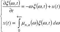
Using the distributed model of ![]() , modeling of the FDE is based on the equations:
, modeling of the FDE is based on the equations:
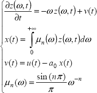
where z(ω, t) is the distributed internal state of ![]() and also the state of the FDE, as in the integer order case.
and also the state of the FDE, as in the integer order case.
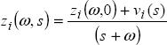
Using the Laplace transform and defining the initial state at t = 0 , i.e. z(ω, 0), we obtain:
Therefore
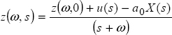
and

Thus

Recall equation [6.16], thus:

The first term of [7.8] corresponds to the system’s free response initialized by z(ω, 0), whereas the second term represents the forced response. This means that the FDE response x(t) is the sum of a free response and a forced response, as in the integer order case [KAI 80, ZAD 08]. The distributed state z(ω, t) is the state of the FDE and also the state of its associated integrator ![]() .
.
The analytical expression of x(t) will be formulated in Chapter 9.
7.3. Closed-loop modeling of an FDS
7.3.1. Modeling of an N-derivative FDS
As any linear FDE can be written as a FDSs, we present the general case of an N -derivative FDS.
Let
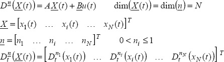
Note that we directly consider the non-commensurate order case.
More specifically, the order ni can be equal to 1, as in the induction motor example presented in Chapter 5.
Note also that it is possible to consider ![]() , with
, with ![]() (so 0 < ni < 1). Thus, it is another reason to introduce integer orders in the model of [7.9].
(so 0 < ni < 1). Thus, it is another reason to introduce integer orders in the model of [7.9].
Obviously, this general model also corresponds to the commensurate order case with ![]() .
.
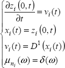
The fractional integrator ![]() associated with the pseudo-state xi (t) corresponds to the equation:
associated with the pseudo-state xi (t) corresponds to the equation:

For ni = 1, these equations are replaced by:
Using the Laplace transform, we can write:
Let us define

and the matrix
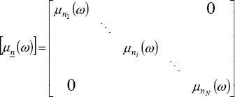
Then
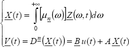
In the Laplace domain, we obtain:

Note that

and

Thus, we can write
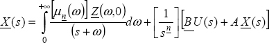
Left multiplication of [7.19] by ![]() and simple calculations yield
and simple calculations yield
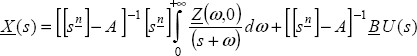
As noted previously, the first term corresponds to the free response initialized by Z(ω, 0), whereas the second term represents the forced response.
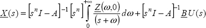
Obviously, equation [7.20] is more simple in the commensurate order case (i.e. ![]() ). Then
). Then
Therefore
The analytical expression of X(t) will be formulated in Chapter 9.
Previous modeling can be qualified as closed-loop modeling, thanks to the closed-loop nature shown in Figure 7.1. However, we can also call it the internal modeling of the FDS, since the state variables zi (ω, t) are those of associated integrators ![]() “inside” the system. The external (or diffusive) representation of FDS will be presented in section 7.7.
“inside” the system. The external (or diffusive) representation of FDS will be presented in section 7.7.
7.3.2. Distributed state
Equations [7.8] and [7.22] can be used to express the distributed state.
For example, consider again the elementary system [7.1] and its step response x(t) caused by u(t) = U H(t) with initial conditions equal to 0, i.e. ![]() .
.
Therefore, we can calculate the components of z(ω, t) at the steady state, i.e. z(ω, ∞):
Thus:
and
Therefore, z(0, ∞) is not defined.
Nevertheless, x(∞) is perfectly defined because
Hence, z(0, ∞) is indirectly characterized by the integral equation:
REMARK 1.– With the frequency discretized model (Chapter 2):
and:

We can also express the components of z(ω, t) when the system is at rest.
Consider the free response caused by z(ω, 0) ≠ 0,
then
which represents the contribution of all the elementary z(ω, 0) frequency components.
Therefore,
Of course, the system is at rest for t → ∞ and:
so we obtain
7.4. Transients of the one-derivative FDS
7.4.1. Numerical simulation
Consider again the elementary system [7.1]:
with a0 = 1 and n = 0.5.
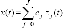
Simulation is performed using equations [7.3].
Practically, a numerical algorithm is used to perform the simulation, where the distributed state variable z(ω, t) is frequency discretized into components zj (t):

Finally, using the Z-transform technique, the complete numerical algorithm is:
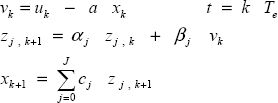
where αj, βj and cj have been defined in Chapter 2 (equations [2.37]–[2.40]).
We consider the following input:
The reference output, using the Mittag-Leffler function (Appendix A.3), is:
where En, 1(−atn) is the Mittag-Leffler function.
The system is simulated with the following parameters:
The reference and simulated outputs are shown in Figure 7.2: as expected and in accordance with Chapter 3, the two curves fit exactly.

Figure 7.2. Comparison of Mittag-Leffler and simulated responses. For a color version of the figures in this chapter, see www.iste.co.uk/trigeassou/analysis1.zip
7.4.2. Initialization at 
In Figure 7.2, we note that x(t) is equal to 0 at the instant t1 = 5.25 s.
Therefore, we propose to initialize the system at t = t1 by imposing u(t) = 0 for t > t1.
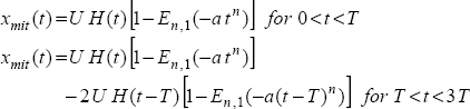
Thus, we modify the computation of xmit (t) for t > t1 , according to:

which corresponds to the equivalent input:
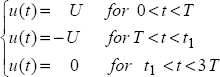
As u(t) = 0 for t > t1, the reference xmit(t) represents the free response of the system for t > t1 , starting from x(t1) = 0 . Hence, we create a reference free response as presented in Figure 7.3.
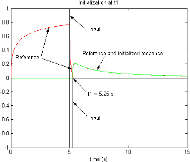
Figure 7.3. Comparison of reference and initialized responses
Moreover, at t = t1, we measure the state z(ω,t1) of the fractional integrator (see Figure 7.5).
Therefore, it is possible to initialize the system, with z(ω, t1) and u(t) = 0 for t > t1.
The initialized response is plotted in Figure 7.3: we can note that the two responses fit perfectly.
The conclusions are as follows:
- – the initial state z(ω, t1) perfectly summarizes the past behavior for t < t1, so the initialized response fits exactly the reference free response for t > t1;
- – the initial state z(ω, t1) corresponds to x(t1) = 0: therefore, we verify that the only knowledge of the pseudo-state variable does not allow the prediction of the fractional system’s free response; it is necessary to refer to its internal state z(ω, t1).
7.4.3. Initialization at different instants
Finally, we consider the following modified input:

The corresponding response x(t) is plotted in Figure 7.4.
Figure 7.4. Initialization at different instants
Figure 7.5 shows the frequency distribution of z(ω, ti ) for these three instants (the index of ω is equal to the index of the discretized frequency ωj , with j varying from 0 to J).
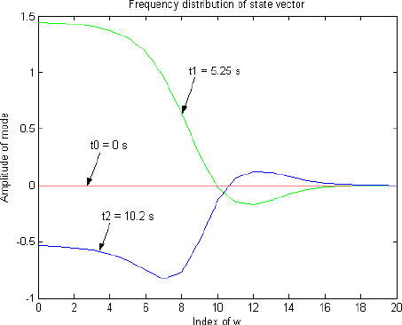
Figure 7.5. Comparison of distributed state vectors
Although the output x(t) has the same value, the three distributions are completely different.
Therefore, the system initialization at each of these instants is represented in Figure 7.4: since the distributed state variables are different, the free responses are of course completely different.
We can conclude that the output x(t) of a fractional integrator is unable to characterize its true state; on the contrary, knowledge of its internal state z(ω,ti ) is required to predict the future behavior.
REMARK 2.– Obviously, these three initializations starting at x(ti ) = 0 are counter examples to the usual belief that the behavior of a fractional system can be characterized by x(ti ) , according to Caputo’s derivative definition (see Chapter 8).
7.5. Transients of a two-derivative FDS
Finally, we consider the two-derivative system:
corresponding to the FDS:
with
The parameters of the two fractional integrators are the same as in section 7.4.1.
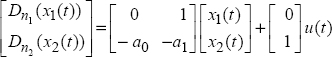
We have considered the step response of this system u(t) = U H(t) U = 1, starting from rest (z1(ω, 0) = 0, z2(ω, 0) = 0). The two variables x1(t) and x2(t) are shown in Figure 7.6.
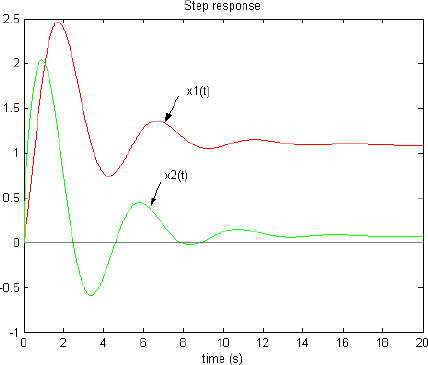
Figure 7.6. Step response of the two-derivative FDS
With a0 = 1, a1 = − 1.2, we verify that there is an oscillatory dominant mode.
The elementary analysis shows that x1(∞) = 1 and x2(∞) = 0: of course, at t = 20 s, these values are not reached (long memory behavior).
Since x1(∞) corresponds to the steady state and x2 (∞) corresponds to rest, we represent z1(ω, t) and z2(ω, t) in Figures 7.7 and 7.8, at the different instants t = 0.5 s, t = 5 s, t = 25 s, t = 250 s.

Figure 7.7. Evolution of z1(ω, t)
We note that z1(ω, t) evolves towards the steady state with z1(0, t) increasing, whereas the other modes converge to zero. For z2(ω, t) , the evolution is towards rest: we note that all the modes converge to zero.
Figure 7.8. Evolution of z2 (ω, t)
Nevertheless, it is important to note that this evolution is very slow (although t = 250 s is a large value, it is far from infinity!), confirming the long-range memory phenomenon.
Moreover, we note that the visualization of the state vectors zi (ω, t) is a good indicator of the system evolution, more significant than the value of the outputs xi (t) .
7.6. External or open-loop modeling of commensurate fractional order FDSs
7.6.1. Introduction
To the best of our knowledge, a non-commensurate order FDS can be modeled only by integrators, so it is necessarily a closed-loop or internal representation. On the contrary, for a commensurate order FDE or FDS, we can calculate the roots of the characteristic equation and the possible poles of the system. Therefore, using the inverse Laplace transform, we obtain a stable multimode and a possible integer order mode, corresponding to each root. Then, the impulse response is the sum of all these modes, and we obtain an external or open-loop representation of the fractional system, also called the diffusive representation of the system [MON 98, HEL 98].
7.6.2. External model of an elementary FDE
Consider again the one-derivative FDE
or equivalently when the system is at rest at t = 0.
Let us define
and
The equation D(s) = sn + a = 0 has a real root λ which verifies
Note that λ is the root of D(s), but it is not the pole of Hn,a(s), as in the integer order case.
Indeed, let us define
and
Then
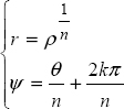
The function sn − λ = 0 is multiform [LEP 80, POD 99]; it requires a cut in the complex plane because we have to respect the constraint:
Recall that λ = −a is real:
- – if a > 0 , then λ < 0 so θ = π + 2kπ and
 with 0 < n < 1
so ![]() and the constraint [7.56] cannot be respected: therefore, there is no pole for a stable FDE;
and the constraint [7.56] cannot be respected: therefore, there is no pole for a stable FDE;
- – on the contrary, if a < 0 , then λ > 0 so θ = π + 2kπ and

which implies ![]() : therefore, there is a positive unstable pole α.
: therefore, there is a positive unstable pole α.
Then, let us calculate the impulse response ![]() using the inverse Laplace transform (see Appendix A.7). We obtain the general expression:
using the inverse Laplace transform (see Appendix A.7). We obtain the general expression:

The first term corresponds to the response of the integer order unstable mode eαt, whereas the second term is a stable aperiodic multimode.
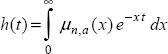
Because there is no pole if a > 0, the impulse response hn,a(t) is only composed of the stable multimode:
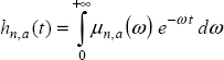
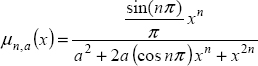
where
REMARK 3.– If a = 0, then ![]() , i.e. we recover the fractional integrator.
, i.e. we recover the fractional integrator.
It is easy to verify that:
Expressions [7.57] and [7.58] are the external impulse responses [ORT 15] of the FDE; they are also known as the diffusive representation of the FDE [MON 98, HEL 98].
Now, consider the response x(t) to any input u(t):
Let ξ(ω, t) be the distributed variable associated with hn , a (t). Then, as with the fractional integrator, we can write:
Let ξ(ω, 0) be the initial condition at t = 0 of system [7.61]. Then
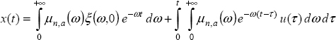
The first term represents the free response, whereas the second term corresponds to the forced response.
Model [7.61] is called external or open-loop because it is not referred to an internal integrator.
Obviously, the distributed variables z(ω, t) (internal state variable) and ξ(ω, t) (external state variable) are completely different.
7.6.3. External representation of a two-derivative FDE
Consider the system
Let λ1 and λ2 be the roots of ![]() .
.
Let ![]() , we can consider the following cases:
, we can consider the following cases:
- – if a0 < 0 , then
 and the roots λ1 and λ2 are real with opposite signs;
 - – if a0 < 0, then Δ > 0 if a1 < 2a0, so λ1 and λ2 are real with the same signs;
- – if a0 < 0, then Δ < 0 if −2a0 < a1 < 2a0.
Then the roots λ1 and λ2 are complex conjugate numbers:

We can also write
With λ1 and λ2, we can write
Now consider the possible poles of ![]() .
.
If λ1 and λ2 are real, it is the same case as noted previously (section 7.2.2).
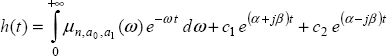
However, if λ1 and λ2 are complex, there are two conjugate poles:
These poles can be expressed as s1 = α+ jβ and s2 = α− jβ with α = cos(ψ) and β = sin(ψ).
They have a negative real part (i.e. they are stable poles) if ![]() , i.e. if
, i.e. if ![]() or
or ![]() . Therefore, we can express the impulse response
. Therefore, we can express the impulse response ![]() using the inverse Laplace transform (see Appendix A.7):
using the inverse Laplace transform (see Appendix A.7):

This important case will be used in Chapter 8 Volume 2 to analyze system stability.
7.6.4. External representation of an N-derivative FDE
Consider the N -derivative commensurate order FDE (or FDS):
In this case, the characteristic equation D(s) has N roots λi that can be real or complex and
These roots λi can correspond to possible poles si.
The impulse response hn, H (t) is the sum of elementary impulse responses as defined in sections 7.6.2 and 7.6.3.
Therefore:
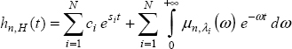
The sum of multimodes gives an equivalent aperiodic multimode, with an equivalent weighting function μn, H (ω).
Therefore, we can write:

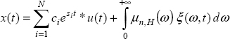
Let ξ(ω, t) be the distributed state variable associated with the equivalent multimode. Then, for any excitation u(t):

Moreover, a response ![]() is associated with each possible integer order pole si.
is associated with each possible integer order pole si.
Therefore, the global forced response x(t) is expressed as:
7.7. External and internal representations of an FDS
We have defined two representations of a fractional system, closed-loop and open-loop (or diffusive). These two representations are equivalent from an input/output point of view.
The open-loop (or external) representation explains the fractional dynamics with the aperiodic multimode, whereas dumped oscillating dynamics are explained by possible integer order conjugate complex poles (for a stable system).
The interest of external representation is to allow direct analysis of system dynamics, particularly to characterize stability with the nature of poles (see Chapter 8, Volume 2).
The closed-loop (or internal) representation does not make it possible to directly characterize system dynamics: it requires numerical simulation or the calculation of the system response with the distributed exponential technique (see Chapter 9).
The external representation requires prior calculation of the roots of D(s) and possible poles, and also of the weighting function μn, H (ω) of the multimode.
On the contrary, the closed-loop representation requires no prior calculation.
Moreover, the external representation requires linearity and commensurability of the FDS. On the contrary, the closed-loop representation is more general because it applies to any FDS, as there is no requirement related to linearity or commensurability.
REMARK 4.– The integer order case corresponds to the commensurate order n = 1. Then, the poles of H(s) coincide with the roots of D(s). Moreover, the multimode vanishes for n = 1. Then, ![]() for n = 1. This means that the external (or diffusive) representation is nothing else than the impulse response representation in the integer order case.
for n = 1. This means that the external (or diffusive) representation is nothing else than the impulse response representation in the integer order case.
REMARK 5.– The closed-loop representation, i.e. modeling using fractional integrators, was defined originally by Trigeassou in a European Control Conference paper in 1999 [TRI 99].
At the same time, and independently, this representation was investigated by Heleschewitz in his PhD [HEL 00]. However, this representation was not developed because the author lacked an efficient approximation technique (infinite gain for ω → 0) for the fractional integrator. Therefore, Heleschewitz focused his works mainly on the analysis of the external representation, called the diffusive representation in his PhD (for more details, see [MON 98, MON 05a, MON 05b, HEL 00]). It was also used by Sabatier [SAB 08b, SAB 10a, SAB 12].
REMARK 6.– In his first monograph [OUS 83], Oustaloup analyzed the time performances of the reference system ![]() step response with a technique based on the inverse Laplace transform, comparable to the diffusive representation, but without the same theoretical background.
step response with a technique based on the inverse Laplace transform, comparable to the diffusive representation, but without the same theoretical background.
7.8. Computation of the Mittag-Leffler function
7.8.1. Introduction
We propose a technique for the computation of the Mittag-Leffler function:
Let us recall the definition of this function (see Appendix A.3):
Truncation of this sum to a large value K >> 1 enables direct computation of this function, as with the exponential function:
However, whereas this computation is independent of t for the exponential function, we note a divergence of the sum for the Mittag-Leffler function occurring for large values of t.
Thus, it is a challenge to propose a computation technique independent of t values. Several techniques have been proposed, for example approaches based on an integral formulation [GOR 02, ORT 17].
We propose to use the equation
where x(t) is the unit step response of the elementary system:
This technique was already proposed by Heleschewitz [HEL 00]; with the same principle, we propose an improved formulation.
7.8.2. Divergence of direct computation
Direct computation is compared to a technique based on the erf function ![]() [KOR 68] for n = 0.5 [HEL 00]:
[KOR 68] for n = 0.5 [HEL 00]:
Figure 7.9 presents the graphs of the two functions for a = 1.
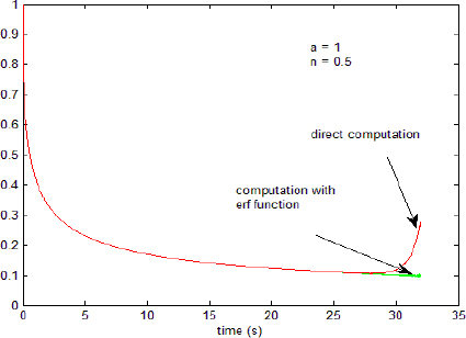
Figure 7.9. Divergence of the Mittag-Leffler function for t > tmax
We verify whether t is limited to a value tmax depending on a (see Table 7.1).
Table 7.1. Divergence of the Mittag-Leffler function versus a , n = 0.5
| a | 0.1 | 1 | 10 |
| tmax (s) | 3000 | 30 | 0.3 |
Note that the computation with the erf function is also divergent for t > tmax.
7.8.3. Step response approach
We first use the computation of x(t) based on the closed-loop representation for the simulation of ![]() . This technique is very easy to implement; however, there is an obvious drawback: in order to obtain En,1(−atn) for the desired value t, it is necessary to recursively compute all the previous values
. This technique is very easy to implement; however, there is an obvious drawback: in order to obtain En,1(−atn) for the desired value t, it is necessary to recursively compute all the previous values ![]() .
.
The graphs of En,1(−atn) and ![]() are plotted in Figure 7.10 with the simulation parameters:
are plotted in Figure 7.10 with the simulation parameters:
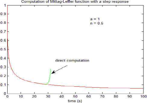
Figure 7.10. Closed-loop computation of the Mittag-Leffler function
We note that the proposed technique enables the computation of the Mittag-Leffler function for t > tmax.
7.8.4. Improved step response approach
We use the same step response technique, but with another formulation of H(s). With the open-loop (or diffusive) representation, we can express H(s) as:
Let u(t) = H(t), then:
As ![]() , we obtain:
, we obtain:

Let us recall that ![]() , thus:
, thus:

Therefore,
Thus,
with

It is essential to note that this approach directly provides the value of the Mittag-Leffler function for the desired value t , without the recursive computation as noted previously.
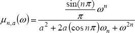
This technique is based on the computation of the integral ![]() . The function μn,a(ω) is precomputed as it does not depend on t . The integral is computed from ωmin to ωmax , with frequencies varying according to a geometric recursion ωj = rωj−1.
. The function μn,a(ω) is precomputed as it does not depend on t . The integral is computed from ωmin to ωmax , with frequencies varying according to a geometric recursion ωj = rωj−1.
Figure 7.11 presents the weighting function μn,a(ω) for n = 0.5, a = 1.
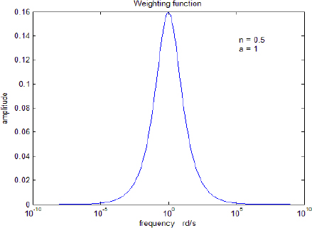
Figure 7.11. Weighting function
We note that ωmin must be chosen close to ![]() whereas ωmax must be very large
whereas ωmax must be very large ![]() with r = 1.04.
with r = 1.04.
Figure 7.12 presents the computation error:

Figure 7.12. Open-loop computation error
This error is maximum for t → 0, and then it decreases ε(t)→0 . The sudden increase at t = 25 s corresponds to the divergence of En,1(−atn).
Figure 7.13 presents the computation of ![]() on the interval [0;100s] for three values of a (0.1 1 10) and for n = 0.5 .
on the interval [0;100s] for three values of a (0.1 1 10) and for n = 0.5 .

Figure 7.13. Mittag-Leffler function for large values of t
All of these graphs highlight that the improved step response technique allows the computation of the Mittag-Leffler function with good accuracy for a > 0, 0 < n < 1 and ![]() .
.
A.7. Appendix: inverse Laplace transform of 
The impulse response of ![]() is calculated using the inverse Laplace transform [SPI 65, LEP 80, POD 99]:
is calculated using the inverse Laplace transform [SPI 65, LEP 80, POD 99]:

with a Bromwich contour, in the same way as ![]() (see Appendix A.6).
(see Appendix A.6).
If a > 0 , there is no pole.
Therefore:
and
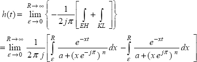
Finally, we obtain
where
On the contrary, if a < 0, there is a pole ![]() inside the Bromwich contour in the positive complex half plane and
inside the Bromwich contour in the positive complex half plane and
which yields:

Note that if a < 0, then eαt is an unstable mode, whereas the multimode remains stable.
REMARK 7.– These results also apply if a is a complex number.
For example, consider
Therefore
where λ1 and λ2 are the roots of H(s) such that:

For each root λ1 or λ2, we can use the previous results, with two complex weighting functions μn,λ1 (ω) and μn,λ1 (ω).
Combining these weighting functions, we obtain a real weighting function ![]() .
.
Finally, using the poles α ± jβ corresponding to λ1 and λ2 , we can express the impulse response as:
Therefore, the impulse response is composed of a stable aperiodic multimode and an integer order oscillatory mode, which is stable if α < 0 or unstable if α > 0.